Accumulations Functions and the Fundamental Theorems of Calculus (Solutions)
The following solutions are for the problems on moments of inertia and rotational energy linked here. I encourage you to attempt them by yourself first before looking through the solutions.
Problem 1
Find the derivatives with respect to $x$ of the following three functions $f(x), g(x), h(x)$:
$$f(x)=\int_0^x e^{-t^2}dt, \quad g(x)=\int_0^{x^2} e^{-t^2}dt, \quad h(x)=\int_x^{x^2}e^{-t^2}dt$$
The derivative of $f(x)$ can be calculated directly using the first FTC.
$$\frac{d}{dx}[f(x)]=\frac{d}{dx}\left[\int_0^x e^{-t^2}dt\right]=e^{-x^2}$$
The derivative of $g(x)$ can be calculated similar using the generalized FTC.
$$\frac{d}{dx}[g(x)]=\frac{d}{dx}\left[\int_0^{x^2} e^{-t^2}dt\right]=e^{-(x^2)^2}\cdot\frac{d}{dx}[x^2]=2xe^{-x^4}$$
Finally, notice that based on the second property of integration, we know that
\[\int_0^{x^2} e^{-t^2}dt=\int_0^x e^{-t^2}dt+\int_x^{x^2}e^{-t^2}dt\]Rearranging this equation gives
\[\int_x^{x^2}e^{-t^2}dt=\int_0^{x^2} e^{-t^2}dt-\int_0^x e^{-t^2}dt\]and using the function definitions given in the problem,
\[h(x)=g(x)-f(x)\longrightarrow \frac{d}{dx}[h(x)]=\frac{d}{dx}[g(x)]-\frac{d}{dx}[f(x)]\]Using our earlier results, we have
$$\frac{d}{dx}[h(x)]=\frac{d}{dx}[g(x)]-\frac{d}{dx}[f(x)]=2xe^{-x^4}-e^{-x^2}$$
Problem 2
This problem is adapted from Bloomsburg University.
Suppose $f$ is the function whose graph is given below.
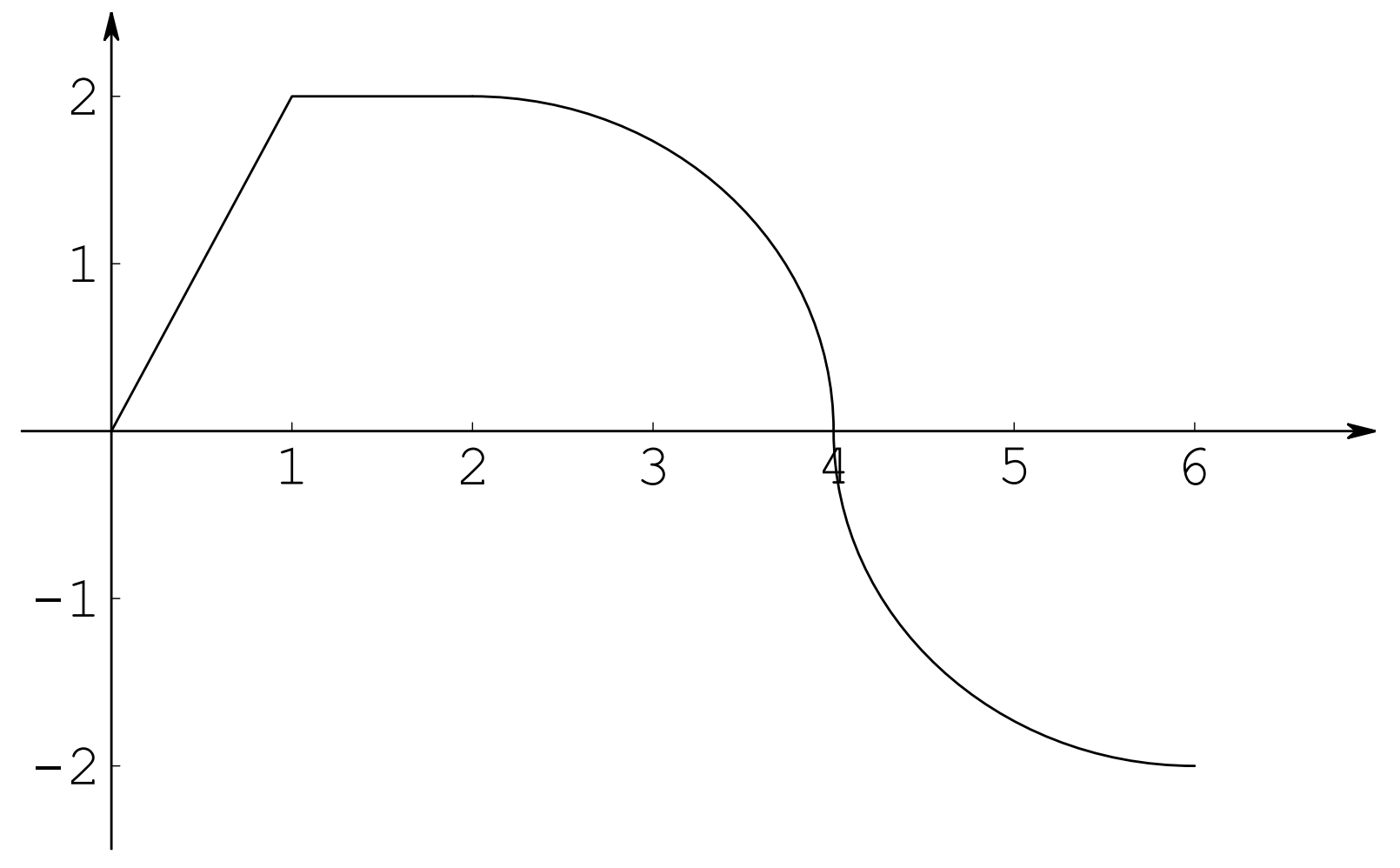
Define the function $g(x)=\int_0^x f(t)dt$.
- Find the values of $g(0), g(1), g(2), g(4), g(6)$.
- Sketch a rough graph of $g(x)$.
Taking inspiration from the example on accumulation functions discussed in the teaching module, we have
$$g(0)=\int_0^0f(t)dt=0$$
$$g(1)=\int_0^1f(t)dt=\frac{1\cdot 2}{2}=1$$
$$g(2)=\int_0^2f(t)dt=\frac{1\cdot 2}{2}+(1\cdot 2)=3$$
$$g(4)=\int_0^4f(t)dt=\frac{1\cdot 2}{2}+(1\cdot 2)+\frac{\pi (2)^2}{4}=3+\pi$$
$$g(6)=\int_0^6f(t)dt=\frac{1\cdot 2}{2}+(1\cdot 2)+\frac{\pi (2)^2}{4}-\frac{\pi (2)^2}{4}=3$$
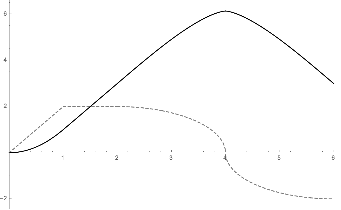
A rough sketch of $g(x)$ is shown here below. $f(x)$ is the gray, dashed line and $g(x)$ is the solid, bold line.
Problem 3
This problem is adapted from Bloomsburg University.
Consider the Fresnel function defined by $$S(x)=\int_0^x \sin\left(\frac{\pi t^2}{2}\right)dt$$ The figures below show the graphs of $y=f(x)=\sin\left(\frac{\pi x^2}{2}\right)$ (dashed line) and $y=S(x)$ (solid line).
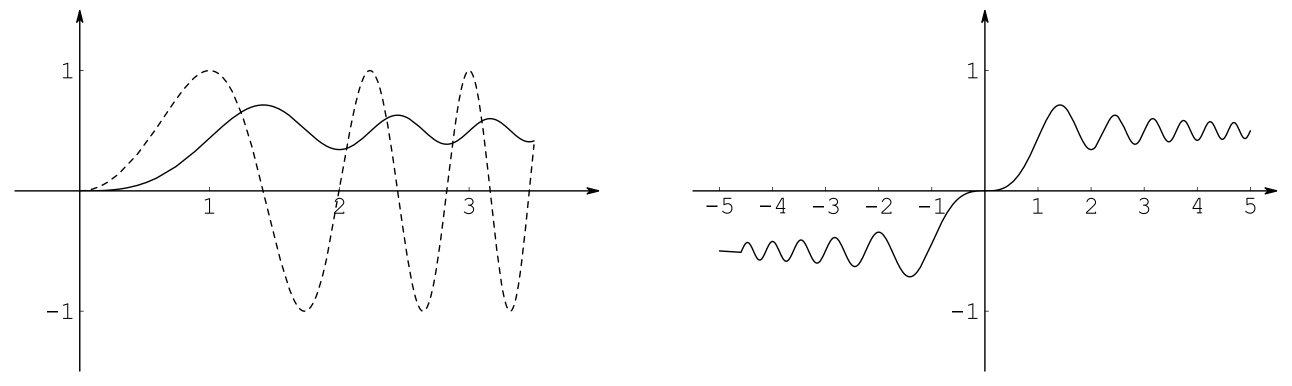
- At what values of $x$ does $S$ have local maximum values?
- On what intervals is the function concave upward?
- Solve the following equation for $x$ correct to at least one decimal place:
$$\int_0^x \sin\left(\frac{\pi t^2}{2}\right)dt=0.2$$
For this problem, only consider the values of $x>0$.
Recall from our discussion on the derivatives of accumulation functions that the accumulation function $S(x)$ has a maximum when the integrand function $f(x)$ goes from positive to negative. By the nature of the sign function, we know that this happens then
\[\frac{\pi x^2}{2}=(2n-1)\pi, \quad n\in\{1, 2, \ldots\}\]Solving for $x$, we get
\[x=\sqrt{2(2n-1)}, \quad n\in\{1, 2, \ldots\}\]Therefore,
The function $S(x)$ has a maximum at $x=\sqrt{2}, \sqrt{6}, \sqrt{10}, \sqrt{14}, \ldots$
Meanwhile, recall that the concavity of $S(x)$ is related to the second derivative of $S(x)$. From the first FTC, we know that the second derivative of $S(x)$ is equal to the first derivative of $f(x)$. $S(x)$ is therefore concave up when the first derivative of $f(x)$ is positive, or in other words, when $f(x)$ is increasing. Therefore, to determine when $S(x)$ is concave up, we look for the intervals when $f(x)$ is increasing.
\[\frac{d}{dx}[f(x)]=\frac{d}{dx}\left[\sin\left(\frac{\pi x^2}{2}\right)\right]=\pi x\cos\left(\frac{\pi x^2}{2}\right)\]This function is equal to zero when
\[\frac{\pi x^2}{2}=\pi\left(n-\frac{1}{2}\right), \quad n\in\{1, 2, \ldots\}\]Solving for the special zeroes gives
\[x=\sqrt{2n-1}, \quad n\in\{1, 2, \ldots\}\]Through inspecting the graph and understanding the nature of the sine function, we know that the $f(x)$ function is increasing when $x$ goes from an even value of $n$ to an odd value of $n$. Therefore, we can conclude that
The function $S(x)$ is concave up on the intervals $x\in[\sqrt{3}, \sqrt{5}]$, $[\sqrt{7}, \sqrt{9}]$, $\ldots$
To solve the last part of this problem, the easiest way to approach this would probably be to use a calculator, as we don’t know how to explicitly evaluate the integral expression for $f(x)$. However, another way to approach this is to recognize that $0.2$ is fairly small, and so we will likely only have to deal with small values of $t$ in the accumulation integral for $S(x)$. Therefore, we can use the small-angle approximation $\sin x\approx x$ to approximate the integral:
\[S(x)=\int_0^x \sin\left(\frac{\pi t^2}{2}\right)dt\approx \int_0^x \frac{\pi t^2}{2}dt\]This approximate integral of a polynomial function is now easy to evaluate:
\[S(x)\approx \left.\frac{\pi}{6}t^3\right\vert_0^x=\frac{\pi x^3}{6}=0.2\]Solving this equation for $x$ gives
$$x=\sqrt[3]{\frac{6}{5\pi}}\approx 0.726$$
For reference, using a calculator to actually solve this problem gives an accurate numerical solution of $x\approx0.738$, so this tells us that our approximation was fairly accurate!