Mechanical Equilibrium: Rotational Motion
Newton’s Laws
In this module, we’ll be continuing to investigate how our working physics framework describes into our current understanding of rotating systems. Let’s review Newton’s laws for rotating systems that we introduced last time:
- If the net torque on an object is zero, the object will remain at constant angular velocity. This means things that are at rest, stay at rest, and things that are rotating continue to move at constant angular velocity.
- The sum of all the torques on an object, $\sum \vec{\tau}$, is called the net torque \(\vec{\tau}_{\text{net}}\), and is given by \(\sum \vec{\tau}=\vec{\tau}_{\text{net}}\propto\vec{\alpha}\), where $\vec{\alpha}$ is the angular acceleration. We will talk about what the proportionality constant exactly is later. (Unlike forces, the proportionality constant is not simply just the mass of the object!)
- For two objects $1$ and $2$ in contact, \(\vec{\tau}_{1\rightarrow 2}=-\vec{\tau}_{2\rightarrow 1}\).
Today, we’ll be talking about systems in mechanical equilibrium and how this relates to these set of laws.
Mechanical Equilibrium
We have talked about what it means for a system to be in mechanical equilibrium before, but our previous definition did not take into account all of our new framework describing the net torque and how it affects the rotations of a system. In order for a system to be in mechanical equilibrium, it still remains true that the system cannot have any linear acceleration, meaning that $\sum \vec{F}=0$ still. However, we also have to assert that the system cannot have any angular acceleration either! This means that things that are rotating shouldn’t suddenly start rotating, and things that are rotating should continue to rotate at a constant angular velocity. This means that we now also have another requirement for mechanical equilibrium: the net torque must also be zero. This now gives us two conditions for mechanical equilibrium that must both be simultaneously satisfied:
$$\sum \vec{F}=0, \quad \sum \vec{\tau}=0$$
Wait a second… if we think back to systems like the inclined plane or the hanging masses, we never talked about the net torque requirement before! Does that mean that our previous physics work was wrong? It turns out that we’re in the clear. The reason why is that in all of our previous physical setups, nothing was ever rotating! There was no axis of rotation or any circular motion, and so the net torque $\sum \vec{\tau}$ was always equal to zero, meaning that this second equilibrium requirement on the net torque was always implicitly satisfied.
Of course, this is not generally the case. If system components have the potential to rotate, then we need to consider the requirement on the net torque a bit more carefully. We’ll talk about some the common problems involving mechanical equilibrium in the context of rotating systems here.
See-Saws
See-saws are common structures that can be found in a lot of playgrounds, and essentially rely on the imbalance of torque applied on either side of the pivot on the see-saw. A standard see-saw problem might look something like this:
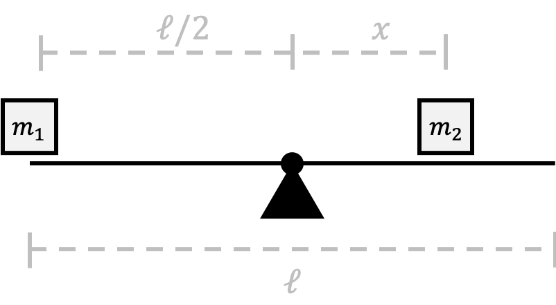
In this setup, we assume arbitrarily that $m_2\geq m_1$, and we want to know where to place $m_2$ on the see-saw such that the see-saw doesn’t rotate or “teeter-totter” to one side or the other. In order words, we need to make sure that the net torque on the see-saw is zero.
What are the sources of torque in this setup? There is the force of gravity acting on $m_1$ and $m_2$ that is also weighing down on the see-saw, in addition to the force of gravity acting on the see-saw itself, and also the normal force $\vec{N}$ from the pivot supporting the see-saw from the center.
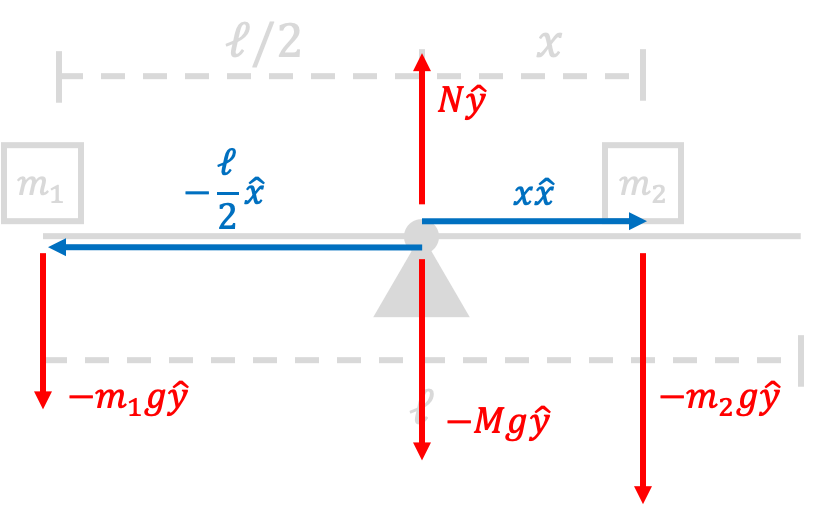
In this diagram, the position vectors $\vec{r}$ are shown in blue, and the force vectors $\vec{F}$ are shown in red. We have also assumed that the mass of the see-saw is $M$, and can be though of as being concentrated completely at the center of the see-saw (we will show that this is a valid assumption when we talk about the center of gravity of objects below). Given this setup with the appropriate parameters, the net torque acting on the see-saw is
\[\sum \vec{\tau}=\vec{\tau}_{m_1}+\vec{\tau}_{m_2}+\vec{\tau}_{M}+\vec{\tau}_{N}\]By the definition of torque, we know that
\[\vec{\tau}_{m_1}=\vec{r}_{m_1}\times\vec{F}_{m_1}=(-1)^2\frac{\ell m_1g}{2}(\vec{x}\times\vec{y})=\frac{\ell m_1g\hat{z}}{2}\]Similarly,
\[\vec{\tau}_{m_2}=-xm_2g(\hat{x}\times\hat{y})=-xm_2g\hat{z}\]In calculating \(\vec{\tau}_{M}\) and \(\vec{\tau}_{N}\), both of the relevant force vectors are being applied at the origin where $\vec{r}=0$, meaning that the magnitude of both of these torque contributions must be zero. Therefore, we can conclude that the net torque is given by
\[\sum \vec{\tau}=\frac{\ell m_1g}{2}\hat{z}-xm_2g\hat{z}\]In order for this system to be in mechanical equilibrium, the net torque must be $0$, and so
\[\frac{\ell m_1g}{2}-xm_2g=0\longrightarrow x=\frac{\ell m_1g}{2m_2g}=\frac{\ell m_1}{2m_2}\]This tells us exactly where to place the second mass $m_2$ relative to the center of the see-saw such that the system remains in mechanical equilibrium and the see-saw does not begin to rotates.
See-Saws (Yes, Again)
In the above example, we seemingly arbitrarily set the origin of our system at the center of the see-saw. Does our answer depend on the fact that our origin is at this particular location?
To investigate this question, let’s instead redefine our origin to be the left-most edge of the see-saw. In this scenario, all of the force quantities remain the same, but the position vectors are now different:
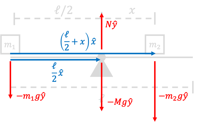
Once again, we have kept the same convention where the position vectors $\vec{r}$ are shown in blue, and the force vectors $\vec{F}$ are shown in red. Given this setup, the net torque acting on the see-saw with respect to this new translated coordinate system is
\[\sum \vec{\tau}=\vec{\tau}_{m_1}+\vec{\tau}_{m_2}+\vec{\tau}_{M}+\vec{\tau}_{N}\]By the definition of torque, we know that
\[\vec{\tau}_{M}=\vec{r}_{M}\times\vec{F}_{M}=-\frac{\ell Mg}{2}(\vec{x}\times\vec{y})=-\frac{\ell Mg\hat{z}}{2}\]Similarly,
\[\vec{\tau}_{N}=\vec{r}_{N}\times\vec{F}_{N}=\frac{\ell N}{2}(\vec{x}\times\vec{y})=\frac{\ell N\hat{z}}{2}\]and
\[\vec{\tau}_{m_2}=-\left(\frac{\ell}{2}+x\right)m_2g(\hat{x}\times\hat{y})=-\left(\frac{\ell}{2}+x\right)m_2g\hat{z}\]Since the force of gravity to $m_1$ is being applied at the origin where $\vec{r}=0$, this means that $m_1$ contributes no torque. Therefore, we can conclude that the net torque is
\[\sum \vec{\tau}=-\frac{\ell Mg}{2}\hat{z}+\frac{\ell N}{2}\hat{z}-\left(\frac{\ell}{2}+x\right)m_2g\hat{z}\]In order for this system to be in mechanical equilibrium, the net torque must be $0$, and so
\[-\frac{\ell Mg}{2}+\frac{\ell N}{2}-\left(\frac{\ell}{2}+x\right)m_2g=0\]At this point, we could solve for $m_2$ in terms of $M$ and $N$. However, what if we want our final answer in terms of $m_1$? In order to rewrite $M$ and $N$ in terms of $m_1$, we need to use the other condition for mechanical equilibrium: the fact that the net force on the see-saw must also be zero. We can use this condition to solve for the magnitude of the normal force $N$ in terms of the other variables in the problem:
\[\sum \vec{F} = N\hat{y}-m_1g\hat{y}-Mg\hat{y}-m_2g\hat{y}\]Because the net force on the see-saw must be zero in mechanical equilibrium,
\[N-m_1g-Mg-m_2g=0\longrightarrow N=(m_1+M+m_2)g\]Substituting this result back into our equation for $x$ from the equilibrium condition on torque, we have
\[-\frac{\ell Mg}{2}+\frac{\ell m_1g}{2}+\frac{\ell Mg}{2}+\frac{\ell m_2g}{2}-\left(\frac{\ell}{2}+x\right)m_2g=0\]Simplifying the left hand side of this equation gives
\[\frac{\ell m_1 g}{2}-xm_2g=0\longrightarrow x=\frac{\ell m_1g}{2m_2g}=\frac{\ell m_1}{2m_2}\]As we can see, this is exactly the same result as we found above! In general, no matter where we set the origin in our problem, we should always arrive at the same answer for physical quantities, such as the position from the center of the see-saw. However, just like what we saw from our previous work in choosing an appropriate coordinate system for the inclined plane problems, some choices for the origin in the problem are better than others. In the first case, we didn’t even have to consider the force balance condition $\sum\vec{F}=0$, and two of the torques didn’t even contribute to the net torque! On the other hand, while doing the same problem the second time around in a different coordinate system was correct, it was arguably much harder.
Different coordinate systems should always lead to the same physical result.
Falling Ladders
Another common mechanical equilibrium setup is a ladder resting against a wall.
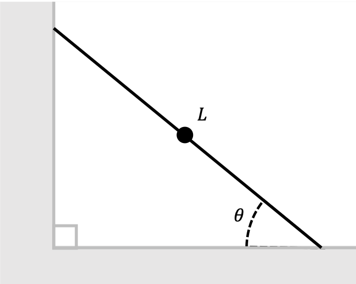
In this example setup, the ladder has some length $L$ and total mass $m$. Similar to the see-saw from above, we will also assume that the mass of the ladder is evenly distributed throughout the entirety of the object, such that we can effectively treat all of the mass as concentrated at the center of the ladder. Intuitively, we know that the force of static friction is holding the ladder up against the well. In this problem, we are interested in determining the minimum angle $\theta$ such that the ladder doesn’t slip and fall. We assume that there is some static coefficient of friction $\mu_s$ between the ladder and the wall/floor.
Just like in the previous problem, we will first construct a force diagram to illustrate the various sources of forces and torques that are acting on the ladder:
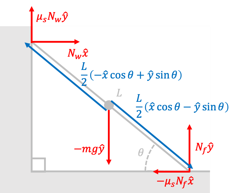
In this diagram above, the position vectors $\vec{r}$ are shown in blue, and the force vectors $\vec{F}$ are shown in red. There are a lot of things happening in this diagram, so let’s break down what is happening.
There are five sources of force that are acting on the ladder simultaneously:
- Gravity: Once again, we are making the assumption that all of the mass is concentrated at the center of the ladder, resulting in a force $-mg\hat{y}$ on the ladder at the origin of our coordinate system.
- Normal Force from the Floor: The floor is supporting the weight of the ladder with a force $N_f\hat{y}$.
- Normal Force from the Wall: The wall is also supporting the ladder with a force $N_w\hat{y}$.
- Static Friction from the Floor: We are interested in the minimum angle before the ladder begins to slip, so the static friction should achieve its maximum amplitude of $\mu_sN_f$ at this particular angle. The ladder is trying to slip “outwards,” and since friction opposes the direction of motion, the force is in the $-\hat{x}$ direction.
- Static Friction from the Wall: By reasoning similar to above, since the ladder is trying to slip “downwards,” the force is in the $+\hat{y}$ direction with magnitude $\mu_sN_w$ by the definition of friction.
The position vectors for where the forces are acting derived from the fact that the total length of the ladder on either side of the origin should be equal and $L/2$. The directional components of the vector are determined through trigonometry in reference to the angle $\theta$ shown in the figure. Given these results, we can define the following torque quantities using the definition of torque $\vec{\tau}=\vec{r}\times\vec{F}$:
\[\vec{\tau}_m=0\] \[\vec{\tau}_{N_f}=\frac{L}{2}(\hat{x}\cos\theta-\hat{y}\sin\theta)\times N_f\hat{y}=\frac{LN_f\cos\theta}{2}\hat{z}\] \[\vec{\tau}_{\mu_sN_f}=\frac{L}{2}(\hat{x}\cos\theta-\hat{y}\sin\theta)\times (-\mu_sN_f\hat{x})=-\frac{\mu_sLN_f\sin\theta}{2}\hat{z}\] \[\vec{\tau}_{N_w}=\frac{L}{2}(-\hat{x}\cos\theta+\hat{y}\sin\theta)\times N_w\hat{x}=-\frac{LN_w\sin\theta}{2}\hat{z}\] \[\vec{\tau}_{\mu_sN_w}=\frac{L}{2}(-\hat{x}\cos\theta+\hat{y}\sin\theta)\times (\mu_sN_w\hat{y})=-\frac{\mu_sLN_w\cos\theta}{2}\hat{z}\]Therefore, given these results and summing all of these contributions, the net torque on the system is
\[\sum\vec{\tau}=\hat{z}\frac{L}{2}\left(N_f\cos\theta-\mu_sN_f\sin\theta-N_w\sin\theta-\mu_sN_w\cos\theta\right)\]Now, using the mechanical equilibrium condition that $\sum\vec{\tau}$, we have
\[N_f\cos\theta-\mu_sN_f\sin\theta-N_w\sin\theta-\mu_sN_w\cos\theta=0\]Solving for $N_f$ in terms of the other parameters in the problem, we find
\[N_f=N_w\frac{\sin\theta+\mu_s\cos\theta}{\cos\theta-\mu_s\sin\theta}\]after simplifying. After considering the torque equilibrium condition, we also need to consider the force equilibrium condition that $\sum\vec{F}=0$, or equivalently, $N_w-\mu_sN_f=0$ for the $\hat{x}$ direction and $\mu_sN_w+N_f-mg=0$ for the $\hat{y}$ direction. Using the $\hat{x}$ direction equilibrium equation, we find that $N_f=\frac{1}{\mu_s}N_w$. When comparing this with the result that we derived using the torque equilibrium constraint, we find that
\[\frac{1}{\mu_s}=\frac{\sin\theta+\mu_s\cos\theta}{\cos\theta-\mu_s\sin\theta}\]From here, it is only a matter of intense algebra to find $\theta$ as a function of $\mu_s$. Dividing the numerator and denominator on the right hand side by $\cos\theta$ gives
\[\frac{1}{\mu_s}=\frac{\tan\theta+\mu_s}{1-\mu_s\tan\theta}\longrightarrow 1-\mu_s\tan\theta=\mu_s\tan\theta+\mu_s^2\]Rearranging both sides gives
\[2\mu_s\tan\theta=1-\mu_s^2\longrightarrow \boxed{\tan\theta=\frac{1-\mu_s^2}{2\mu_s}}\]This equation gives us the minimum angle $\theta$ in terms of $\mu_s$ before the ladder begins to slide off of the wall and floor, as desired.
Center of Gravity
In both of the example exercises above, we asserted that although gravity was acting on the entirety of the see-saw and the ladder, we could simply concentrate all of the torque contribution as if the plank’s weight were concentrated at the center. Let’s prove that this is the case. Consider the following setup:
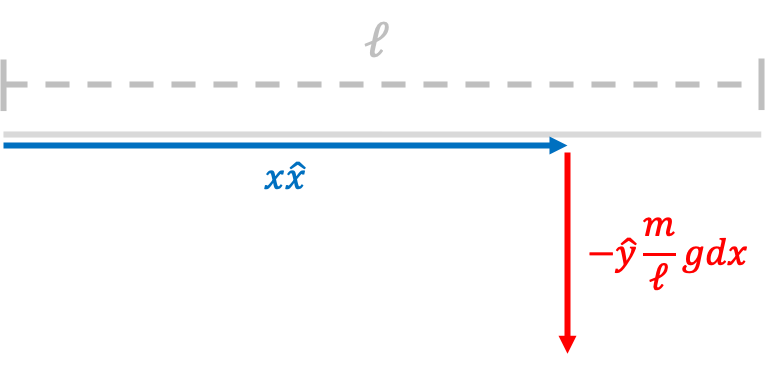
In this setup, we are choosing the origin to be the left end of the rod, and we have some sort of one-dimensional rod is horizontal and has an equal mass density distribution throughout the entirety of the rod. The total mass of the rod is $m$ and the total length of the rod is $\ell$, and so a small segment of the rod of length $dx$ has a total mass of $\frac{m}{\ell}dx$. Therefore, the force of gravity acting on their small rod segment is $d\vec{F}=-\hat{y}\frac{mgdx}{\ell}$.
The torque on this small rod segment, which we shall denote as $d\vec{\tau}$, is given by
\[d\vec{\tau}=\vec{r}\times d\vec{F}=x\hat{x}\times \left(-\hat{y}\frac{mgdx}{\ell}\right)=-\frac{xmgdx}{\ell}\hat{z}\]Integrating all of the torque contributions along the entirety of the rod gives us the total torque $\vec{\tau}$:
\[\vec{\tau}=-\hat{z}\int_0^\ell dx\frac{x mg}{\ell}=-\hat{z}\frac{mg}{2\ell}x^2\vert_0^\ell=-\hat{z}\frac{mg\ell}{2}\]after simplification. Note that this is exactly the same as the torque contribution from a single, point mass of mass $m$ a distance $\ell/2$ from the origin. This tells us that our assumption that we used in the previous two problems to concentrate all of the mass in calculating the torque due to gravity is valid. (We didn’t prove this result for a slanted rod, such as a ladder, but it is not hard to imagine that this conclusion still holds. In Problem 2 of the exercises below, you will prove that this result holds for any angle $\theta$.)
Based on simply using our intuition, we are often able to guess the location of the center of gravity.
The center of gravity of a homogeneous, symmetric body must lie on the axis of symmetry.
In this context, “homogeneous” means that the mass of the object is evenly distributed throughout the entirety of the volume of the object. For example, the center of gravity of a homogeneous sphere is its center, and the center of gravity of a homogeneous rectangular prism is where its three axes of symmetry meet.
In general, this point of application of a single force of magnitude $F_g=mg$, where $m$ is the total mass of the object, is called the object’s center of gravity. In one dimension, the center of gravity position $\vec{x}_{\text{cog}}$ is defined by the equation
\[(m_1g+m_2g+m_3g+\cdots)x_{\text{cog}}=m_1gx_1+m_2gx_2+m_3gx_3+\cdots\]where $m_1, m_2, m_3, \ldots$ are the masses of the individual particles that make up the object, and $x_1, x_2, x_3$ are the positions of the corresponding particles relative to the origin. This equation is derived by equating the torque exerted by the force $F_g$ at the center of gravity to the sum of the torques acting on the individual particles. Solving for $x_{\text{cog}}$ gives
\[x_{\text{cog}}=\frac{m_1x_1+m_2x_2+m_3x_3+\cdots}{m_1+m_2+m_3+\cdots}=\frac{\sum_i m_ix_i}{\sum_i m_i}\]This gives the $x$-coordinate of the center of gravity. The $y$- and $z$- coordinates of the center of gravity of the system can be found in a similar way.
\[y_{\text{cog}}=\frac{\sum_i m_iy_i}{\sum_i m_i}, \quad z_{\text{cog}}=\frac{\sum_i m_iz_i}{\sum_im_i}\]Of course, these formulas only apply if the system can be divided into a finite set of discrete, point-like masses. A continuous mass distribution requires more complicated integral calculus in multiple dimensions, which is far beyond the scope of our discussion here.
Exercises
Problem 1
Consider the following configuration of three masses:
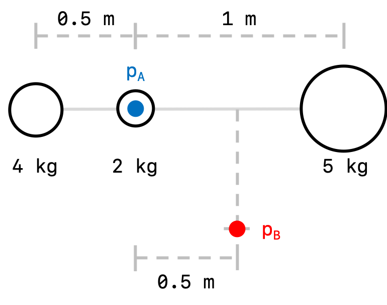
Answer the following two questions:
- What are the $(x, y)$ coordinates of the center of gravity of this system when $p_A$ is taken at the origin?
- What are the $(x, y)$ coordinates of the center of gravity of this system when $p_B$ is taken at the origin?
Problem 2
Consider a homogenous, one-dimensional rod of mass $m$ and length $\ell$ that makes an angle $\theta$ with the $x$-axis.
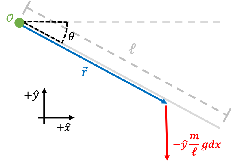
Similar to the exercise above in the notes, show that, with respect to the origin $\mathcal{O}$ (highlighted in green), the torque due to all of the force of gravity acting on center of gravity is equal to the torque due to the force of gravity acting throughout the entirety of the rod.
Problem 3
This problem is adapted from Serway Physics 9ed.
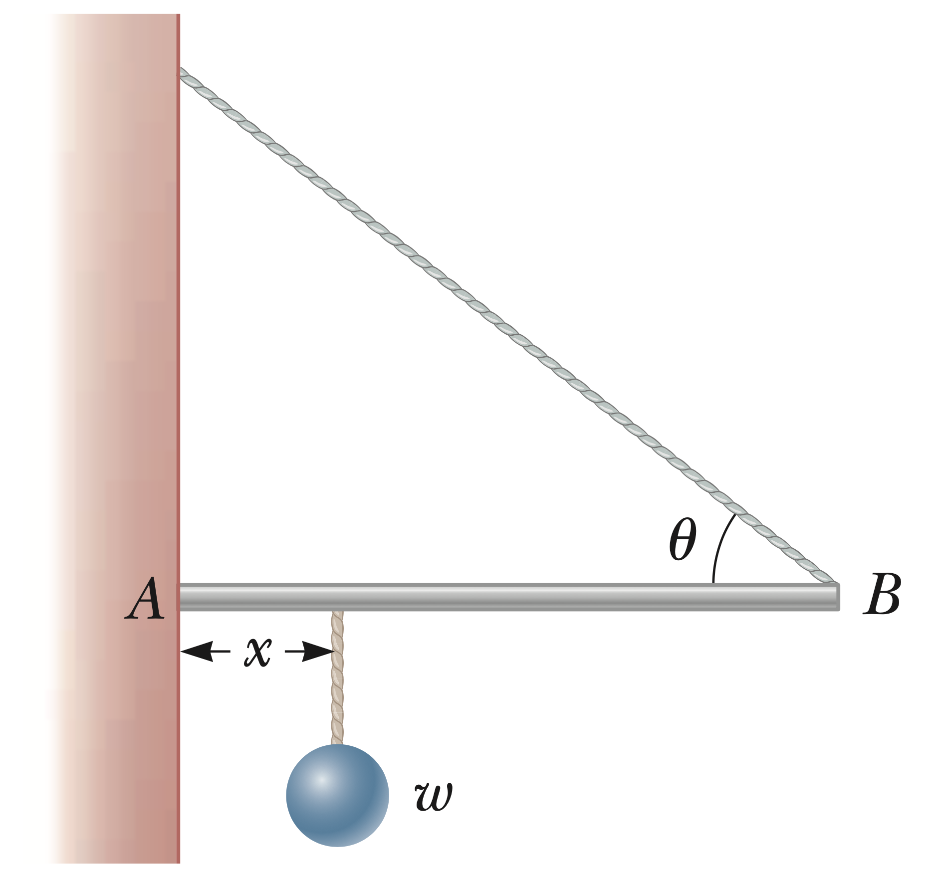
One end of a uniform 4 meter long rod of mass $m$ is supported by a cable at an angle of $\theta=\pi/4$ with the rod. The other end rests against a wall, where it is held by friction. The coefficient of static friction between the wall and the rod is $\mu_s=0.5$. Determine the minimum distance $x$ from point $A$ at which an additional weight of mass $m$ (the same as the mass of the rod) can be hung without causing the rod to slip at point $A$.
Problem 4
Suppose two children are using a uniform seesaw that is 3 m long and has its center of mass over the pivot. The first child has a mass of 30 kg and sits 1.4 m from the pivot.
- Calculate where the second child, who has a mass of 18 kg, must sit to balance the seesaw.
- What is unreasonable about this result? What needs to be changed in the initial problem setup so that a reasonable result can be obtained?