Introduction to Derivatives
Last time, we asked the question of what happens when we want to find the slope of a secant lint between two points $(x, f(x))$ and $(x+h, f(x+h))$ for some parameter $h$. The slope $m$ of this secant line is
\[m=\frac{f(x+h)-f(x)}{h}\]Today, we’ll see what happens as we take the limit as $h\rightarrow 0$. That is, what happens when the two points begin to approach each other? To think about this problem, let’s go back to Problem 3 from last time, where we considered the function $f(x)=x^2$. Let’s evaluate the slope $m$ from above for this function:
\[m=\frac{(x+h)^2-x^2}{h}=\frac{x^2+2xh+h^2-x^2}{h}=\frac{2xh+h^2}{h}=2x+h\]We’re interested in what happens in the limit as $h\rightarrow 0$. In this case, this limit is pretty easy to evaluate:
\[\lim_{h\rightarrow 0}m=\lim_{h\rightarrow 0}(2x+h)=2x+0=2x\]What is this statement telling us? As $h\rightarrow 0$, the secant line starts to become the tangent line that is tangent to the curve $f(x)$ at a particular value of $x$. We call this a tangent line because locally, it only intersects $f(x)$ at one point. The slope of this tangent line is called the derivative. Based on our calculations from above, the derivative, which we’ll denote as $m$ for now, is defined to be
\[m=\lim_{h\rightarrow 0}\frac{f(x+h)-f(x)}{h}\]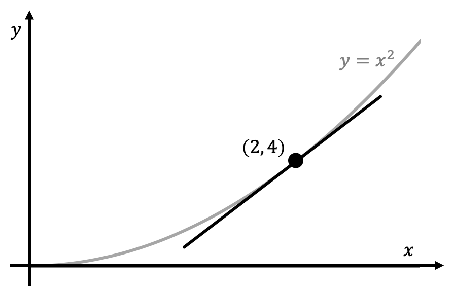
The above figure illustrates an example of a tangent line that is tangent to the curve $f(x)=x^2$ at the point $(2, 4)$. Based on our formula from above, the slope of this tangent line at this point is $m=2(2)=4$. Since we know that the point $(2, 4)$ lies on this tangent line, we could use the point-slope formula to then write down the explicit form of the tangent line. This is just an illustrative example of what a derivative is: the derivative describes the slopes of tangent lines to a curve $f(x)$.
Derivative Notation
In reality, derivatives aren’t denoted as $m$. There are two common ways to denote the derivative of a function $f(x)$: (1) prime notation and (2) Leibniz notation. Prime notation looks like this:
\[f'(x)=\lim_{h\rightarrow 0}\frac{f(x+h)-f(x)}{h}\]The presence of a $’$ symbol denotes that we’re taking the derivative of the function. Leibniz notation looks like this:
\[\frac{df}{dx}=\frac{d}{dx}[f(x)]=\lim_{h\rightarrow 0}\frac{f(x+h)-f(x)}{h}\]For reasons that we’ll talk about later, I highly recommend you use the Leibniz notation, but you should be familiar with and able to read/use both types of derivative notations.
Properties of the Derivative
Fundamentally, a derivative is defined as a limit. This means that many properties about limits can also apply to derivatives:
- In order for a derivative to exist, it shouldn’t matter whether we approach the limit from the left or from the right. In other words, the limit must be defined from either direction. This makes sense, since we know that that $\lim_{x\rightarrow c}$ only exists when the limits $\lim_{x\rightarrow c^-}$ and $\lim_{x\rightarrow c^+}$ are equal. As an example, the derivative at $x=0$ of $f(x)=\vert x\vert$ does not exist. In general piece-wise discontinuous functions (like a step function) and functions with sharp edges (like an absolute value function).
- A derivative can only exist then the function is defined there. For these reasons, rational functions like $1/x$ have an undefined derivative at $x=0$, and $\sin(1/x)$ also has an undefined derivative at $x=0$.
- For the above reasons and a few more, we can arrive at a pretty substantial conclusion:
Differentiability implies continuity.
This statement means that if a function is differentiable at some point $x=x_0$, then we are guaranteed that the function is also continuous at the same point $x=x_0$. This also means that if we know that the function is not continuous at a given point, it must also not be differentiable at that point too. However, note that the converse is not true: if the function is continuous at some point $x=x_0$, it does not necessarily mean that the function is is also differentiable at that same point.
Differentiability Implies Local Linearity
Let’s go back to the first graph of this page where we plotted the function $y=x^2$ and the tangent line of this function at the point $(2, 4)$. Imagine that we zoomed in really close to this particular point $(2, 4)$. Although the tangent line and actual function aren’t necessarily equal, they do look very similar. This can often be used to our advantage to approximate function values that would otherwise be difficult to evaluate. Let’s say that we know the derivative of a function, and also a point that lies on the function:
\[df/dx\text{ and }f(a)=b\text{ are given and for some }a, b\]Using this information, we can derive a linear approximation for the function that’s pretty good close to the point $(a, b)$ on the graph.
\[y-a=\left.\frac{df}{dx}\right\vert_{x=a, y=b}(x-b)\]The slope in the point-slope notation here is the derivative $df/dx$ evaluated at the particular point $(a, b)$. This result is called the tangent line approximation and can be used to approximate values of $y$ near $x=a$.
Visualizing Derivatives
A very common type of problem asks you to graph both $f(x)$ and $df/dx$ on the same graph given one versus the other. There are three rules involving the first derivative that you should know:
- If $df/dx>0$ at a particular point, then $f(x)$ is increasing at that point.
- If $df/dx<0$ at a particular point, then $f(x)$ is decreasing at that point.
- If $df/dx=0$ at a particular point, then $f(x)$ has a critical point at that point.
A rather unhelpful, but technically correct, definition of a critical point is a point where the first derivative is equal to zero. A more practical definition is a critical point is a local extremum (meaning minimum or maximum) or a saddle point. Here are three of the most common examples for critical points:

Let’s go over a simple example to illustrate this. Consider the following graph of the derivative of \(f(x)\):
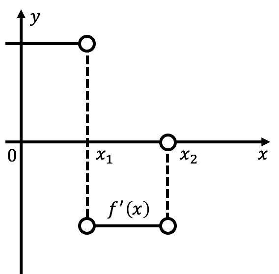
Our goal is to sketch what \(f(x)\) looks like given this graph of \(f'(x)\). For $x<x_1$, $f’(x)$ is just some constant positive number, meaning that $f(x)$ is increasing by the same amount all the time irregardless of the value of $x$ we’re at, so long as $x<x_1$. This corresponds to an increasing linear function. For $x_1\leq x<x_2$, $f’(x)$ is a constant negative number, and so by similar reasoning, this corresponds to a decreasing linear function. For $x\geq x_2$, $f’(x)=0$, and so the function $f(x)$ isn’t decreasing or increasing: it is just remaining at some constant value since its rate of change is zero. Therefore, superimposing the graphs of $f(x)$ and $f’(x)$ together, we might have something that looks like
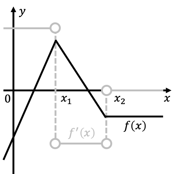
We’ll be able to further improve our graph function sketches once we introduce the notion of the second derivative. Sketching either $f(x)$ or $f’(x)$ (or both) involves practice to get a strong intuition about how functions and their derivatives behave.
Mean Value Theorem
The mean value theorem for derivatives (MVT) is a commonly cited theorem in calculus. Assume that we have a function $f(x)$ that satisfies the following two properties:
- $f(x)$ is continuous on the closed interval $[a, b]$.
- $f(x)$ is differentiable on the open interval $(a, b)$.
The mean value theorem states that if $f(x)$ satisfies both of these properties, then there must exist at least one point $x=c$ with $a<c<b$ such that
\[f'(c)=\frac{f(b)-f(a)}{b-a}\]What is theorem saying? Consider the arbitrary polynomial function shown below:
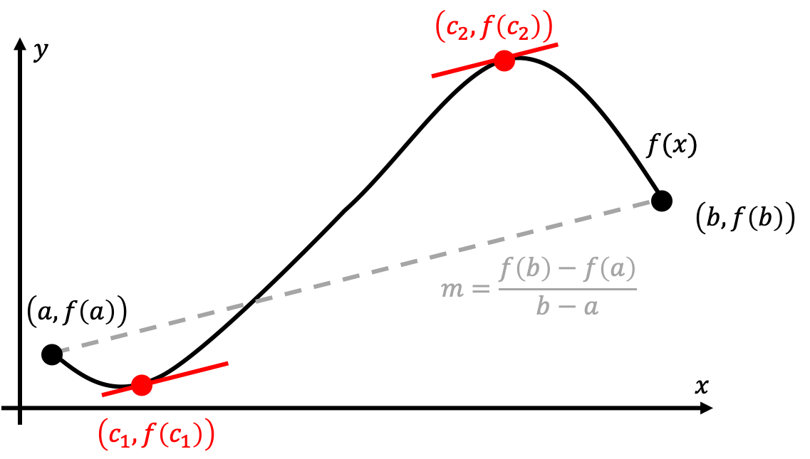
MVT essentially guarantees the existence of at least one point (or in our case, two points $x=c_1$ and $x=c_2$) such that the derivative(s) at the point(s) is equal to the average rate of change along the entirety of the curve. In the figure above, we can see that the two red points have tangent slopes that are parallel to the average slope along the curve, which is highlighted in gray. As we can see, MVT can be though of as the “derivative version” of the intermediate value theorem.
Rolle’s Theorem
Rolle’s Theorem is essentially MVT in the very special case where $f(a)=f(b)$, and $a<b$. Defined more explicitly, assume that we have a function $f(x)$ defined on the interval $a\leq x\leq b$, with the properties that
- $f(x)$ is continuous on the closed interval $x\in[a, b]$.
- $f(x)$ is differentiable on the open interval $x\in(a, b)$.
- $f(a)=f(b)$ and $a<b$.
If $f(x)$ satisfies all three of these properties, then direct application of MVT that we learned above tells us that there exists at least one point $x=c$ with $a<c<b$ such that $f’(c)=0$, since the numerator of $\frac{f(b)-f(a)}{b-a}$ is equal to zero. This is Rolle’s Theorem. An visual diagram is shown here:
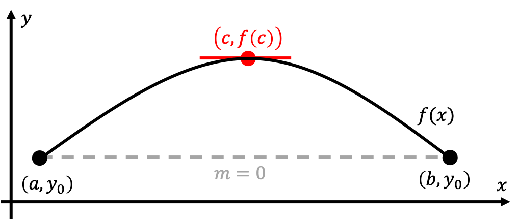
In this diagram, $y_0=f(a)=f(b)$, and so we are guaranteed the existence of the highlighted red point $(c, f(c))$ with derivative given by $f’(c)=0$ using Rolle’s Theorem.
Exercises
Problem 1
Earlier, we asserted that just because a function is continuous at a given point does not mean that it is also differentiable at that same point. Give two different examples of shapes of functions that are continuous at at least one point, but not differentiable at that point.
Problem 2
Consider the function $f(x)$ that we graphed above in our discussion involving using the piecewise constant $f’(x)$ function to sketch $f(x)$. This function can also be the derivative of another function, which we can denote as $F(x)$. That is, $dF/dx=f(x)$. Using our sketch of $f(x)$ above, sketch out the general shape of $F(x)$.
Problem 3
Consider a function $y=f(x)$ with a derivative given by
\[\frac{df}{dx}=x-y-2\]At $x=-1$, $y$ is known to be $3$.
- Using this information, construct a tangent line approximation of the value of $y$ near $x=-1$.
- It is known that the actual value of $y$ at $x=-0.9$ is $y(-0.9)\approx 2.434$. How good is your approximation at $x=-0.9$?
- It is known that the actual value of $y$ at $x=0$ is $y(0)=-3+7e^{-1}\approx -0.425$. How good is your approximation at $x=0$?
Problem 4
This problem is adapted from the 2007 AP Calculus AB Exam.
Let $f$ be a twice-differentiable function such that $f(2)=5$ and $f(5)=2$. Let $g$ be the function given by $g(x)=f(f(x))$.
- Explain why there must be a value $c$ for $2<c<5$ such that $f’(c)=-1$.
- Show that $g’(2)=g’(5)$. Use this result to explain why there must be a value $k$ for $2<k<5$ such that $g’‘(k)=0$. Note: You must be familiar with the chain rule before attempting this subproblem. If you haven’t seen this yet, skip this part of the problem.
- Show that if $f’‘(x)=0$ for all $x$, then the graph of $g$ does not have a point of inflection. Note: You must be familiar with higher order derivatives before attempting this subproblem. If you haven’t seen this yet, skip this part of the problem.
- Let $h(x)=f(x)-x$. Explain why there must be a value $r$ for $2<r<5$ such that $h(r)=0$.
Problem 5
Suppose we know that $f(x)$ is continuous and differentiable on the interval $[-7, 0]$, that $f(-7)=-3$, and that $f’(x)\leq 2$ for the entirety of that interval. What is the largest possible value for $f(0)$?