Introduction to Integration
We’ll going to entirely switch gears now and move onto the next big topic that follows differentiation: integration (we’ll define what this is below). To motivate this discussion let’s consider the following situation.
A Motivating Example
Let’s consider the following graph:
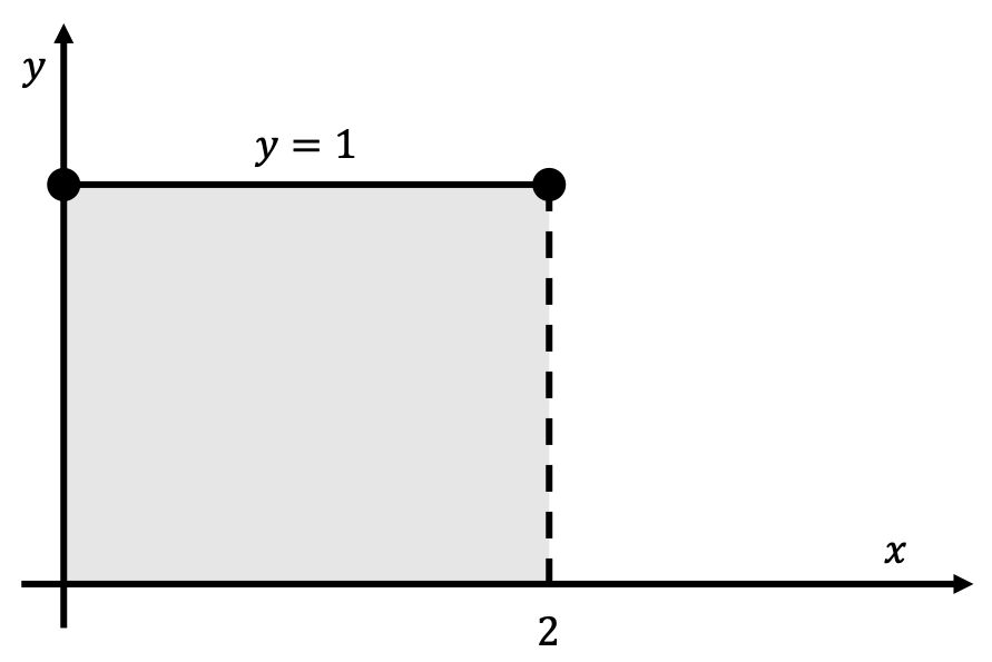
Here, we’re considering the constant function $y=f(x)=1$ on the interval $0\leq x\leq 2$. Let’s assume that we want to find the area underneath this curve between the curve (or in this case, or the straight line) and the $x$-axis (in other words, the gray area shaded in the figure above). In this simple case, we can use simple geometry to figure out the area underneath the curve. This is a rectangle with length 2 and height 1, so the area is simply $A=(2)(1)=2$ squared units. This example isn’t super interesting, largely because this is a common and simple geometric figure that’s easy to take the area under. Let’s say that instead, we had the following graph:

How can we take the area underneath this arbitrary curve? There’s no simple geometric formula to apply here, so we need to figure out a more general way of taking areas under functions.
Areas Under Arbitrary Functions: A Picture
From above, we know taking the area under an arbitrary function is very difficult, but taking the area under a rectangle is very easy (it’s just length multiplied by the height, as we saw above). So, if we could somehow convert this problem into multiple “sub-problems” of finding the area of rectangles instead, then this problem might be more approachable. For example, consider the following diagram:
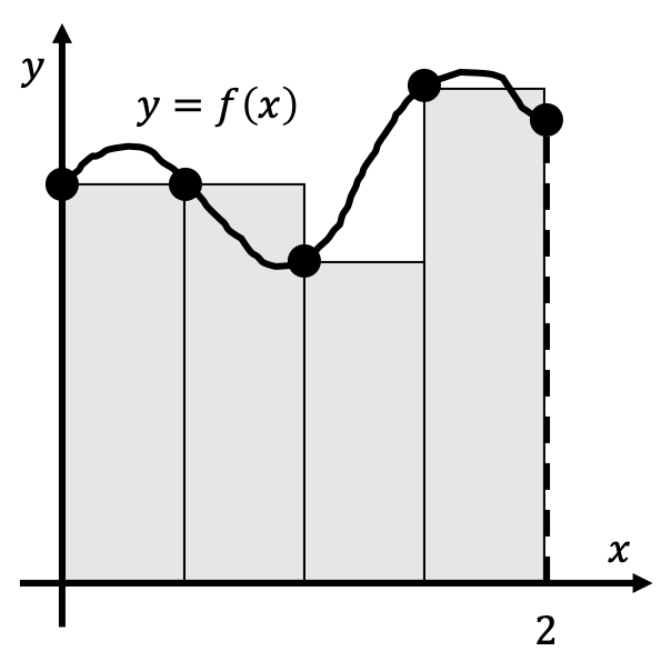
What we did here was break down the area underneath the curve into small pieces that can be approximated as rectangles. In some cases, the rectangles underestimate the area underneath the curve (for example, the first and the third rectangles), and in other cases, the rectangles overestimate the area underneath the curve (for example, the second rectangle in the figure above). In order to approximate the total area underneath the curve $y=f(x)$ on the interval $0\leq x\leq 2$, we can just calculate the area of all of these different rectangles and then sum them all together.
Of course, these doesn’t look like a great approximation for the area. What if we split up the interval into more than just four rectangles? The result might look something like this:
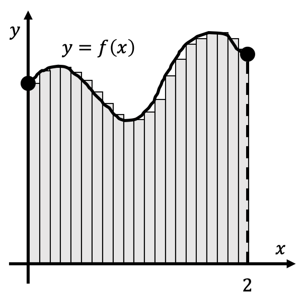
Now, it seems like summing over the areas of the individual rectangles is a much better approximation for the actual area under the curve $y=f(x)$. In general, you can imagine that as we increase the number of rectangles, our approximation for the area under the curve gets better and better, and as that number of rectangles increases to $\infty$, the approximation becomes an exact expression for the area under the curve. This gives us an algorithm for to approach how to figure out finding the area under an arbitrary curve.
Areas Under Arbitrary Functions: An Algorithm
Now that we have a better idea of how we can approach finding the area under a curve, and we need to know how to write this approach mathematically. Consider again the problem of some arbitrary function:
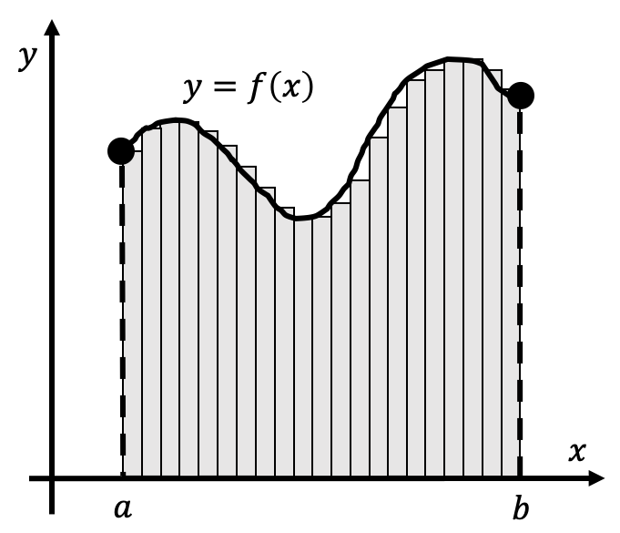
This time, we’re considering a function $y=f(x)$ on the interval $a\leq x\leq b$ for some $a, b$ with $a<b$. Let’s consider the case where we’ve partitioned our interval into $n$ number of rectangles. Each of our rectangles have an equal width, and the total length of the $x$ interval is $b-a$, meaning that each of the rectangles have a width $(b-a)/n$.
The height of each of the rectangles is a bit more difficult to consider. Let’s first number the rectangles going from the left to right from $1$ to $n$. At the $i$th rectangle, the left edge of the rectangle is at the $x$ coordinate $x=a+\frac{(b-a)(i-1)}{n}$ (feel free to check this as well), while the right edge of the rectangle is at the $x=a+\frac{(b-a)i}{n}$. In the above diagrams, we determined the height of the $i$th rectangle through the $y$ value of the left edge of the rectangle, which we know to be $y=f\left(a+\frac{(b-a)(i-1)}{n}\right)$. Therefore, we can conclude that the area contribution of the $i$th rectangle is given by
\[A_i=\text{width}\times\text{height}=\frac{b-a}{n}\cdot f\left(a+\frac{(b-a)(i-1)}{n}\right)\]Now, all we have to do is sum over all of the areas for all of the $n$ rectangles to get the total area under the curve. This gives us the following expression:
\[\text{Area Under }f(x)\approx \sum_{i=1}^n \left[\frac{b-a}{n}\cdot f\left(a+\frac{(b-a)(i-1)}{n}\right)\right]\]Since $b, a, n$ are all just constants with respect to $i$, so we can rewrite this as
\[\text{Area Under }f(x)\approx \frac{b-a}{n}\sum_{i=1}^n f\left(a+\frac{(b-a)(i-1)}{n}\right)\]This is our expression for the area under the curve.
Example
To show an example of how we can use this algorithm, let’s consider the function $y=f(x)=x^2$ on the interval $1\leq x\leq 2$, with $n=5$ rectangles to be used to approximate the area underneath the curve.
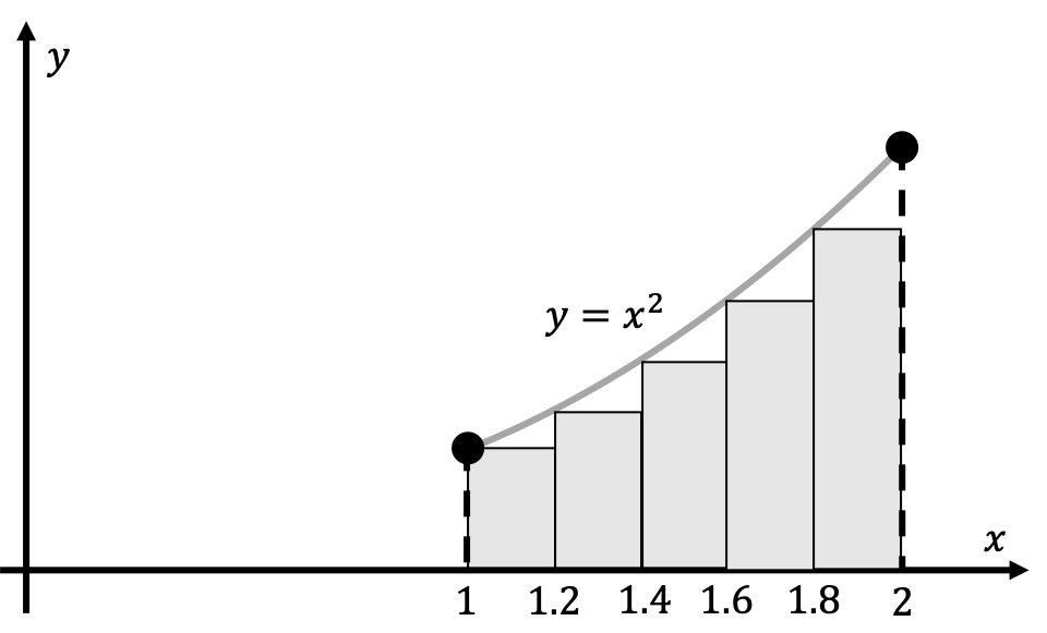
Here, we know that
\[a=1, b=2, n=5 \longrightarrow \frac{b-a}{n}=\frac{1}{5}\]Therefore, we have the following table of $x$ values:
| $i$ | 1 | 2 | 3 | 4 | 5 |
| $x=a+\frac{(b-a)(i-1)}{n}$ | 1 | 1.2 | 1.4 | 1.6 | 1.8 |
| $f\left(a+\frac{(b-a)(i-1)}{n}\right)$ | 1 | 1.44 | 1.96 | 2.56 | 3.24 |
Applying our approximation for the area under the curve from above, we find
\[\text{Area Under }f(x)\approx\frac{1}{5}(1)+\frac{1}{5}(1.44)+\frac{1}{5}(1.96)+\frac{1}{5}(2.56)+\frac{1}{5}(3.24)\]We can evaluate the right hand side of this expression using a calculator to get
\[(\text{Area Under }f(x)\text{ where }1\leq x\leq 2)\approx 2.04\text{ square units}\]Ultimately, we will learn how to easily calculate the are under this curve explicitly, and will find that the exact area underneath the curve is $7/3\approx 2.33$, so it looks like our approximation for the area wasn’t too bad using this method!
Other Methods of Approximating Area Under Curves
Summing over $n$ rectangles each with a height determined as a function of the $x$ coordinate of their left edge (i.e. the algorithm that we defined above) is called the left Riemann sum approximation. It is named after Bernhard Riemann, a German mathematician that essentially invented this idea. However, there are also other methods that you might also encounter to approximate area under curves. We’ll discuss some of the common ones here.
Right Riemann Sum
From the name, you might be able to guess that a right Riemann sum is the same as a left Riemann sum except that the right edge of the rectangle is used to determine the height of the individual rectangles instead of the left edge. From above, we determined that the right edge of the $i$th rectangle is given by $x=a+\frac{(b-a)I}{n}$. Therefore, our approximation for the area under $f(x)$ on the interval $a\leq x\leq b$ using $n$ rectangles is given by
\[\text{Area Under }f(x)\approx \frac{b-a}{n}\sum_{i=1}^n f\left(a+\frac{(b-a)i}{n}\right)\]We can try out an example problem by considering the same example from above. Namely, consider the function $y=f(x)=x^2$ on the interval $1\leq x\leq 2$, with $n=5$ rectangles used to approximate the area underneath the curve.
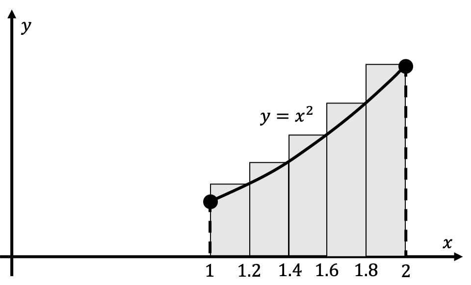
Once again, we have
\[a=1, b=2, n=5 \longrightarrow \frac{b-a}{n}=\frac{1}{5}\]We also have the following table of $x$ values:
| $i$ | 1 | 2 | 3 | 4 | 5 |
| $x=a+\frac{(b-a)i}{n}$ | 1.2 | 1.4 | 1.6 | 1.8 | 2.0 |
| $f\left(a+\frac{(b-a)i}{n}\right)$ | 1.44 | 1.96 | 2.56 | 3.24 | 4 |
Applying our right Riemann sum approximation, we find
\[\text{Area Under }f(x)\approx\frac{1}{5}(1.44)+\frac{1}{5}(1.96)+\frac{1}{5}(2.56)+\frac{1}{5}(3.24)+\frac{1}{5}(4)=2.64\]Again, this isn’t that far off from the actual area value of the region, which is about $2.33$.
Midpoint Riemann Sum
As we saw when using both the left and right Riemann sums, these algorithms can sometimes result in under-approximating or over-approximating a lot of the individual rectangles. The midpoint Riemann sum can sometimes help with this. The idea is that when determining the height of a particular rectangle, we use neither the left nor the right edge: we use the average of the two $x$ coordinates instead. As we discussed, the left edge of the $i$th rectangle is given by $x=a+\frac{(b-a)(i-1)}{n}$, while the right edge of the $i$th rectangle is given by $x=a+\frac{(b-a)i}{n}$. Therefore, the average of the two is given by
\[x_{\text{mid}}=\frac{\left(a+\frac{(b-a)(i-1)}{n}\right)+\left(a+\frac{(b-a)i}{n}\right)}{2}=a+\frac{(b-a)(2i-1)}{2n}\]Therefore, our approximation for the area under $f(x)$ using $n$ rectangles using the midpoint Riemann sum is given by
\[\text{Area Under }f(x)\approx \frac{b-a}{n}\sum_{i=1}^n f\left(a+\frac{(b-a)(2i-1)}{2n}\right)\]Again, to illustrate this, consider the same function $y=x^2$ on the interval $1\leq x\leq 2$, with $n=5$ rectangles used to approximate the area underneath the curve.

| $i$ | 1 | 2 | 3 | 4 | 5 |
| $x=a+\frac{(b-a)(2i-1)}{2n}$ | 1.1 | 1.3 | 1.5 | 1.7 | 1.9 |
| $f\left(a+\frac{(b-a)i}{n}\right)$ | 1.21 | 1.69 | 2.25 | 2.89 | 3.61 |
Therefore, our approximation using the midpoint Riemann sum is
\[\text{Area Under }f(x)\approx\frac{1}{5}(1.21)+\frac{1}{5}(1.69)+\frac{1}{5}(2.25)+\frac{1}{5}(2.89)+\frac{1}{5}(3.61)=2.33\]Comparing this with actual the actual area of the region, we see that this is an extremely good approximation!
Trapezoidal Riemann Sum
The final area-finding algorithm that we’re going to discuss is called the trapezoidal Riemann sum. The idea behind it is that instead of using rectangles to approximate the individual area segments, let’s use trapezoids instead. This might be confusing, so let’s consider our canonical example first. Here’s what the picture might look like.
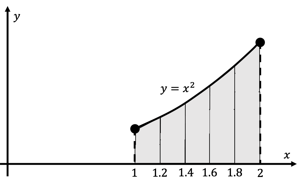
The area of each of the individual trapezoids is equal to the width multiplied by the average height, as we’ve learned from geometry. The average height is given by
\[h_{\text{avg}}=\frac{f\left(a+\frac{(b-a)(i-1)}{n}\right)+f\left(a+\frac{(b-a)i}{n}\right)}{2}\]Applying this formula to our five trapezoids, we have
| $i$ | 1 | 2 | 3 | 4 | 5 |
| $x=a+\frac{(b-a)(i-1)}{n}$ | 1 | 1.2 | 1.4 | 1.6 | 1.8 |
| $x=a+\frac{(b-a)i}{n}$ | 1.2 | 1.4 | 1.6 | 1.8 | 2.0 |
| $f\left(a+\frac{(b-a)(i-1)}{n}\right)$ | 1 | 1.44 | 1.96 | 2.56 | 3.24 |
| $f\left(a+\frac{(b-a)i}{n}\right)$ | 1.44 | 1.96 | 2.56 | 3.24 | 4 |
| $h_{\text{avg}}$ | 1.22 | 1.70 | 2.26 | 2.90 | 3.62 |
Therefore, using the trapezoidal Riemann sum, we have the following approximation:
\[\text{Area Under }f(x)\approx\frac{1}{5}(1.22)+\frac{1}{5}(1.70)+\frac{1}{5}(2.26)+\frac{1}{5}(2.90)+\frac{1}{5}(3.62)=2.34\]From this exercise, we can generalize to get that the trapezoidal Riemann sum formula is given by
\[\text{Area Under }f(x)\approx \frac{b-a}{2n}\sum_{i=1}^n \left[f\left(a+\frac{(b-a)(i-1)}{n}\right)+f\left(a+\frac{(b-a)i}{n}\right)\right]\]Defining the Integral
As we said above, our graphical picture leads us to expect that as $n$ increases, our approximation for the area under a curve gets better and better until it is no longer an approximation: it’s an exact expression. We can therefore define the exact equation:
\[\text{Area Under }f(x)=\lim_{n\rightarrow \infty} \frac{b-a}{n}\sum_{i=1}^n f\left(a+\frac{(b-a)(i-1)}{n}\right)\]One last thing: how we’re denoting the left hand side is a bit cumbersome, as we don’t want to keep writing the phrase “Area Under $f(x)$” all the time in our work. At this point, its a good idea to introduce new notation: the integral notation. By definition, the integral of the function $f(x)$ from $x=a$ to $x=b$ is the area under the curve $y=f(x)$ between $x=a$ and $x=b$, and is denoted by the following:
\[\int_a^b dx\text{ }f(x)=\lim_{n\rightarrow \infty} \frac{b-a}{n}\sum_{i=1}^n f\left(a+\frac{(b-a)i}{n}\right)\]The $\int$ symbol can be though of as a summation symbol similar to $\sum$, except that $\int$ will sum over the a continuous set of intervals of $x$, rather than a discrete set of intervals. The lower bound of integration is $x=a$, and the upper bound of integration is $x=b$. These are denoted as a subscript and superscript on the $\int$ symbol, respectively. $dx$ can be though of as the infinitesimally small width of the rectangles that we’re summing over, and $f(x)$ is the height of the each of the rectangles that we’re summing over. So, $f(x)dx$ is essentially the width of the rectangle multiplied by the height of the rectangle at some particular value of $x$ within the interval $a\leq x\leq b$.
It’s also worthwhile to note that we defined the integral using a limit on the right Riemann sum, but there’s no reason why we couldn’t also define the integral using the left Riemann sum, or the midpoint Riemann sum, or the trapezoidal Riemann sum, or really any other summation algorithm. In reality, all of these approximation techniques will approach the same result if we take the limit as $n\rightarrow \infty$, so it doesn’t really matter which one we choose.
Example
Let’s go back to our classic example we’ve seen multiple times above where we’re trying to find the exact area under the curve $y=f(x)=x^2$ within the interval $1\leq x\leq 2$. Using the definition of the integral that we defined above, we can write the following
\[\int_1^2dx\text{ }x^2=\lim_{n\rightarrow \infty}\frac{2-1}{n}\sum_{i=1}^{n}\left(1+\frac{(2-1)i}{n}\right)^2\]We can simplify the expression on the right hand side:
\[\int_1^2dx\text{ }x^2=\lim_{n\rightarrow \infty}\frac{1}{n}\sum_{i=1}^{n}\left(1+\frac{2i}{n}+\frac{i^2}{n^2}\right)\]We can divide up the sum to get
\[\int_1^2dx\text{ }x^2=\lim_{n\rightarrow \infty}\left[\frac{1}{n}\sum_{i=1}^n 1+\frac{2}{n^2}\sum_{i=1}^{n}i+\frac{1}{n^3}\sum_{i=1}^n i^2\right]\]Use the summation formulas at the bottom of this page to rewrite each of the remaining sums:
\[\int_1^2dx\text{ }x^2=\lim_{n\rightarrow \infty}\left[\frac{1}{n}(n)+\frac{2}{n^2}\frac{n(n+1)}{2}+\frac{1}{n^3}\frac{n(n+1)(2n+1)}{6}\right]\]The final step is to take all of the appropriate limits based on our previous work on limits at infinity:
\[\int_1^2dx\text{ }x^2=1+1+\frac{2}{6}=\frac{7}{3}\]Therefore, we can conclude that the exact area underneath the curve $y=x^2$ between the interval $1\leq x\leq 2$ is $\frac{7}{3}$ squared units, as desired.
Of course, this seems to be a very tedious and mathematically difficult method of determining areas, but it’s a start. Similar to our work with derivatives, now that we have established the fundamentals, we can start working on developing a toolkit of rules and calculus techniques that will allow us to more easily evaluate these these integrals without going through this limit definition every time. We’ll delve deeper into this idea next time in the next lesson.
Wrap Up
We started out today by asking us the simple question of how to find the area under some arbitrary curve. One way of accomplishing this is by breaking up the area of the curve into smaller areas that can be approximated as rectangles (or some other geometric figure). We determined the following four algorithms for approximating the area under a curve $y=f(x)$ between the interval $a\leq x\leq b$ using $n$ rectangles:
- Left Riemann Sum: \(\int_a^b dx\text{ }f(x)\approx \frac{b-a}{n}\sum_{i=1}^n f\left(a+\frac{(b-a)(i-1)}{n}\right)\)
- Right Riemann Sum: \(\int_a^b dx\text{ }f(x)\approx \frac{b-a}{n}\sum_{i=1}^n f\left(a+\frac{(b-a)i}{n}\right)\)
- Midpoint Riemann Sum: \(\int_a^b dx\text{ }f(x)\approx \frac{b-a}{n}\sum_{i=1}^n f\left(a+\frac{(b-a)(2i-1)}{2n}\right)\)
- Trapezoidal Riemann Sum: \(\int_a^b dx\text{ }f(x)\approx \frac{b-a}{2n}\sum_{i=1}^n \left[f\left(a+\frac{(b-a)(i-1)}{n}\right)+f\left(a+\frac{(b-a)i}{n}\right)\right]\)
The exact area under the curve can be found by taking any one of the right sides to $n\rightarrow \infty$. For example,
\[\int_a^b dx\text{ }f(x)=\lim_{n\rightarrow \infty} \frac{b-a}{n}\sum_{i=1}^n f\left(a+\frac{(b-a)(i-1)}{n}\right)\]This expression is called the integral of $f(x)$ from $x=a$ to $x=b$.
Exercises
Problem 1
- Approximate the area under the curve $f(x)=x^2+2$ on the interval $-2\leq x\leq 1$ with a Riemann sum, using six sub-intervals and right endpoints.
- Approximate the area under the curve $f(x)=\sqrt{x+1}$ on the interval $-1\leq x\leq 0$ with a Riemann sum, using four sub-intervals and midpoints.
- Approximate the value of the integral $f(x)=\int_1^3 (x^3-3)dx$ with a Riemann sum, using three sub-intervals and left endpoints.
Problem 2
In the algorithms that we explored today, we assumed that each of the sub-intervals for the $n$ rectangles were of equal width. However, there is no reason why that absolutely must be the case. Using the following table data, use some form of Riemann sum (your pick) to approximate the following integral expression.
\[\int_0^{13}dx\text{ }f(x)\]| $x$ | 0 | 5 | 8 | 10 | 12 | 13 |
| $f(x)$ | 5 | 7 | 6 | 8 | 7 | 8 |
Do the same thing to approximate this integral, but using a different Riemann sum algorithm this time (again, of your choice):
\[\int_0^{16}dx\text{ }g(x)\]| $x$ | 0 | 2 | 5 | 8 | 13 | 16 |
| $g(x)$ | 6 | 4 | 6 | 7 | 8 | 9 |
Problem 3
Use the left Riemann sum-based definition of the integral to evaluate each of these integral expressions:
- \[\int_1^4 dx\text{ }(2x+3)\]
- \[\int_0^1 dx\text{ }[6x(x-1)]\]