Sorting Algorithms, Part 1: The Basics
As we discussed previously, the prerequisite that a list is sorted is essential in order for us to be able to search through it using a faster algorithm such as binary search. In the following two sections, we will discuss efficient (and inefficient) algorithms that can be used to satisfy this prerequisite and sort lists/arrays of elements.
A Brute Force Attempt: Straight Insertion Sort
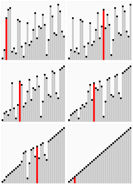
Straight insertion sort is perhaps the most basic method to sort a given list. The idea is to create a new list and add elements one by one in a sorted order. Here is a GIF illustrating how the straight insertion sort algorithm works, taken from this link:

A standard Java implementation of this algorithm might look something like this:
public static List<Integer> straightInsertionSort(List<Integer> toSort) {
    ArrayList<Integer> sorted = new ArrayList<>();

    /* Iterate over every element in the original list. */
    for (int i = 0; i < toSort.size(); i++) {
        boolean placed = false;

        /* Iterate backwards through the sorted list. */
        for (int j = sorted.size() - 1; j >= 0; j--) {
            /* If the element we're currently sorting is at least
             * the current element but less than the element to the
             * immediate right, then insert it at the current position.
             */
            if (toSort.get(i) >= sorted.get(j)) {
                sorted.add(j + 1, toSort.get(i));
                placed = true;
                break;
            }
        }

        /* If the element we're currently sorting is smaller than
         * all of the current elements in the sorted array, then
         * add the element to the beginning of the list.*/
        if (!placed) { sorted.add(0, toSort.get(i)); }
    }

    return sorted;
}
Another Simple Algorithm: Bubble Sort
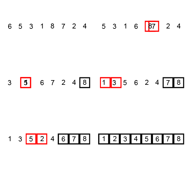
Bubble sorting is a method in which the larger values in the array “bubble up” to the top (meaning the end) of the array. Basically, it works by repeatedly swapping adjacent elements if they are in the wrong order. We continuously make these swaps over and over again and continue to iterate through the entire list until we can make one entire iteration through the list without any swaps in order to know that the list is now sorted. Illustrating GIFS taken from Wikipedia are shown here.


A standard Java implementation of this algorithm might look something like this:
public static List<Integer> bubbleSort(List<Integer> toSort) {
    ArrayList<Integer> sorted = (ArrayList)toSort.clone();

    boolean isSorted = false;

    /* So long as the list is not sorted... */
    while (!isSorted) {
        isSorted = true;

        /* Iterate over every single element of the list. */
        for (int i = 0; i < sorted.size() - 1; i++) {
            /* If the current element is not sorted relative
             * to its right neighbor...
             */
            if (sorted.get(i) > sorted.get(i + 1)) {
                /* ...swap the two neighboring elements. */
                int temp = sorted.get(i);
                sorted.set(i, sorted.get(i + 1));
                sorted.set(i + 1, temp);
                isSorted = false;
            }
        }
    }

    return sorted;
}
It turns out that while both bible sorting and straight insertion sorting are (relatively) easy algorithms to implement, they are not particular efficient and take quite a while to run for large data sets. In the sections below, we’ll discuss more efficient algorithms to sort different lists.
Quicksort
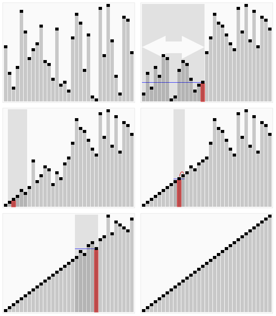
Quick sort is a much faster sorting algorithm that uses recursion to divide the array into smaller and smaller sub-arrays that can be more easily sorted. The basic algorithm is
- Pick a pivot element.
- Partition the array elements into two categories: either less than pivot or greater than the pivot.
- Repeat until the array is sorted.
To summarize, the quicksort algorithm can be broadly separated into two steps: pivot and partition. A good GIF that illustrates this algorithm from Wikipedia is shown here.

Pivot
The pivoting element can be thought of as a “reference value” that is important for the next partition step. There are a number of different common ways to pick the pivot:
- Always pick the first element of the list as the pivot.
- Always pick the last element of the list as the pivot.
- Pick some random element in the array as the pivot.
- Pick the median as the pivot.
Pivot choices 1 and 2 are by far the most common. In our implementation of quicksort below, we will use method 2 to choose our pivot.
Partition
The partition component “pivots” all of the elements in the list around the chosen pivot, such that all of the elements smaller than the pivot are to the left and all of the elements larger than the pivot are to the right. Here is some “pseudo-code” that illustrates what the partition function should look like:
partition(list, low, high) {
    /* Choose the pivot to be the last element in the list. */
    pivot = list[high];

    /* Index to begin adding the elements smaller than the pivot. */
    smallIndex = low - 1;

    /* Iterate over all of the elements in the list. */
    for (i = low; i < high; i++) {
        if (list[i] < pivot) {
            smallIndex++;
            // swap list[smallIndex] and list[i]
        }
    }

    /* After moving all of the smaller elements to the left, put
     * the pivot immediately to the right.
     */
    // swap list[smallIndex + 1] and list[high]

    /* Return index of pivot. */
    return smallIndex + 1;
}
In terms of actual Java code, this is a typical implementation of the partition() function.
public static int partition(int[] list, int low, int high) {
    /* Choose the pivot to be the last element in the list. */
    int pivot = list[high];

    /* Index to begin adding the elements smaller than the pivot. */
    int smallIndex = low - 1;

    /* Iterate over all of the elements in the sub-list. */
    for (int i = low; i < high; i++) {
        /* Move smaller elements to the left of the pivot. */
        if (list[i] < pivot) {
            smallIndex++;
            int temp = list[smallIndex];
            list[smallIndex] = list[i];
            list[i] = temp;
        }
    }

    /* After moving all of the smaller elements to the left, put
     * the pivot immediately to the right.
     */
    int temp = pivot;
    list[high] = list[smallIndex + 1];
    list[smallIndex + 1] = temp;

    /* Return the index of the pivot in the sorted subarray. */
    return smallIndex + 1;
}
Putting it All Together
Once we have our pivot selection and partition function methods setup, writing the quicksort algorithm is actually really easy. The idea is that we continuous quicksort the elements to the left of the pivot and to the right of the pivot over and over again recursively. In Java, this can be implemented in the following method:
public static void quickSort(int[] toSort) {
    quickSort(toSort, 0, toSort.length - 1);
}

private static void quickSort(int[] toSort, int low, int high) {
    if (low < high) {
        /* Pivot the array between low and high around the pivot. */
        int pivotIndex = partition(toSort, low, high);

        /* Quicksort the array less than the pivot. */
        quickSort(toSort, low, pivotIndex - 1);
        /* Quicksort the array greater than the pivot. */
        quickSort(toSort, pivotIndex + 1, high);
    }
}
Notice that we have implemented this method as a public-private pair. Furthermore, notice that in contrast to the previous two methods from above, this particular implementation actually changes the original unsorted array instead of creating a new sorted array. We chose to implement this algorithm in this way simply because it’s easier to do.
Merge Sort
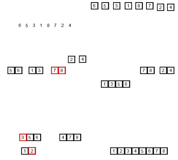
The merge sort algorithm essentially works by breaking down a list into its singular units and then “merges” these building blocks together to create the finalized list. Here is a nice GIF from Wikipedia that illustrates how this algorithm works:

Explicitly listing out the steps to the algorithm:
- Divide the array into two equal halves.
- Call
mergeSort()recursively on the first half. - Call
mergeSort()recursively on the second half. - Merge the two halves sorted in steps 2 and 3.
To summarize, the merge sort algorithm can be broadly separated into two steps: merge and sort.
Merge
The merge step merges two subarrays that are right next to each other in the original array. In the process of merging the two subareas, the final output array is still maintained in a sorted order. A Java implementation of the merge function can look something like this
/** Merge two subarrays arr[l] to arr[m] and arr[m + 1] to arr[r]. **/
public static void merge(int[] arr, int l, int m, int r) {
    /* Create temporary copies of the two subarrays. */
    int[] left = Arrays.copyOfRange(arr, l, m + 1);
    int[] right = Arrays.copyOfRange(arr, m + 1, r + 1);

    /* Variables to store current index in the sorting process. */
    int lIndex = 0;
    int rIndex = 0;

    /* Sort the array arr from arr[l] to arr[r]. */
    for (int j = l; j < r + 1; j++) {
        /* If there's nothing in the left array, then take
         * from the right array.
         */
        if (lIndex >= left.length) {
            arr[j] = right[rIndex];
            rIndex++;
        }
        /* If there's nothing in the right array, then take
         * from the right array.
         */
        else if (rIndex >= right.length) {
            arr[j] = left[lIndex];
            lIndex++;
        }
        /* If the left element is less than the right element,
         * then add the left element to the array.
         */
        else if (left[lIndex] <= right[rIndex]) {
            arr[j] = left[lIndex];
            lIndex++;
        }
        /* If the right element is less than the left element,
         * then add the right element to the array.
         */
        else {
            arr[j] = right[rIndex];
            rIndex++;
        }
    }
}
Sort
The sort step is the main function that recursively breaks down the array and then merges the resulting subarrays using the merge() function that we wrote above. A Java implementation of the merge function looks something like this:
public static void sort(int[] toSort) {
    sort(toSort, 0, toSort.length - 1);
}

private static void mergeSort(int[] toSort, int low, int high) {
    if (low < high) {
        /* Calculate the middle index. */
        int mid = low + ((high - low) / 2);

        /* Sort the first and second halves. */
        mergeSort(toSort, low, mid);
        mergeSort(toSort, mid + 1, high);

        /* Merge the halves. */
        merge(toSort, low, mid, high);
    }
}
Divide and Conquer Algorithms
The merge sort and quicksort algorithms we discussed above are examples of divide and conquer algorithms. This class of algorithms work by recursively breaking down a problem into two or more sub-problems of the same or related type, until they become simply enough to be solved directly. When then combined the solutions to the sub-problems all together to give a solution to the original problem. Divide and conquer algorithms turn out to be some of the most efficient algorithms out there. We will encounter more of them in the future.
Additional Sorting Algorithms
We have only explored a few of the many different sorting algorithms out there. Of course, there are more advanced variations and complex algorithms for sorting, but these are the basics. If you’re interested in learning more, I encourage you to check out this link here.
A Cool Video
To conclude, there’s a pretty cool YouTube video that illustrates the different sorting algorithms that we’ve talked about here (in addition to other ones that we haven’t talked about). I encourage you to watch up to around the 1 minute 30 second mark. (The audio is a bit weird and doesn’t add too much to the video, so maybe mute the video though.)
Exercises
Problem 1
Read about the stability of different sorting algorithms in this Wikipedia link here. Based on your understanding of stability and the different sorting algorithms that we have learned about which of them are stable and which are unstable? (You can find the solution here in the “Which sorting algorithms are stable?” section around the middle of the page.)
Problem 2
By running the program below, compare the time efficiency of the four sorting algorithms that we discussed above in sorting a random array of integers. What do you notice about their relative behaviors? (Note: For the default list size of numElements = 50000, the program takes about 2 minutes to run, so be patient. Feel free to change numElements to explore the relative behaviors of either larger or smaller data sets. Make sure to read over the code as well so that you’re familiar with what is going on. Click on the little ![]() icon at the top left in the plugin to look over all of the different sorting algorithm implementations.)
icon at the top left in the plugin to look over all of the different sorting algorithm implementations.)