Introduction to Electrostatics
In this module, we will begin learning the second major topic of AP Physics: electromagnetism. As we will see, electromagnetism (abbreviated as E&M) is the study of electric and magnetic fields and how they interact with different types of matter. Electromagnetism is often considered to be the most difficult field of physics at the introductory level, but hopefully, we’ll be able to make the learning process as painless as possible.
Our discussion will begin with electrostatics, which is the study of the electric fields and forces between stationary charged particles.
Preface
Just as calculus is the language of Newtonian mechanics, linear algebra and multivariable calculus is the language of electromagnetism. While it is somewhat common for students learning about classical mechanics to maybe have some level of familiarity with calculus, it is very rare for students learning about electromagnetism to have a corresponding understanding of the mathematical tools necessary to understand electricity and magnetism.
Therefore, we will attempt to discuss topics in electromagnetism without assuming any knowledge more than perhaps one-dimensional calculus. However, we’ll still include appropriate derivations using the advanced mathematical formalism needed to derive important results in E&M. This optional derivations and additional notes based in an understanding of linear algebra and multivariable calculus will be highlighted in orange, and can be skipped if the student doesn’t require the level of advanced rigor (which is basically 98% of the time).
Electromagnetism is also all about using symmetry. Often times, the mathematics that we encounter in electromagnetism are hairy and complex. However, we can often simplify it greatly by making some arguments about what the answer should look like based on some underlying symmetry of the problem. Especially in the exercises, we will see many instances where we don’t have to do any work at all (aside from some basic arithmetic) to arrive at the correct answer.
Charge
In order to talk about electricity, we need to first talk about charge. Like mass, charge is some sort of fundamental quantity associated with all types of matter. We have often experienced what electric charge is in our everyday lives. For example, if you rub an inflated rubber ballon against wool, the balloon will then stick to the wall of a room. This is because the balloon becomes electrically charged when it rubs against wool.
The phenomenon of electric charge was mainly derived through actual physics experiments. For example, experiments from the eighteenth century demonstrated that there are two kinds of electric charge, which we know term as positive and negative charge. From experimental observations, we know that
Like charges repel one another and unlike charges attract one another.
This means that two positively charged objects will repel one another, just as two negatively charged objects will repel one another. However, a positively charged object will attract a negatively charged object (and vice versa).
It’s also important to note that just because we call negative charge as “negative” doesn’t mean that there is anything essentially negative about it. It is not like a negative integer, for example: a negative integer differs fundamentally from a positive integer in that its square is an integer of opposite sign. However, the product of two charges is not a charge, and so this definition of “negative” doesn’t really translate well to negative charges. The convention to call certain charges “negative” and the other charge type as “positive” is really more of a historical convention (physicists aren’t perfect!).
It is important to note that charge is quantized. This means that there is a fundamental unit of charge measurements, which we will denote as $e$, and we can’t have fractional units of charge. In other words, the only allowed values of charge is $ne$, where $n$ is an integer. We can’t have $0.5e$ or $0.22e$ worth of charge. (It turns out that in particle physics, charge quantization can actually be violated, but for the purposes of electromagnetism we’re not interested in that here.)
Another important feature of charge is that it is conserved. This means that for a given isolated system, the amount of charge stays the same. It may pass from object to object, but the net charge of the isolated system is a constant.
Coulomb’s Law
The interaction between two charged objects is dictated by Coulomb’s law, which essentially states that two stationary electric charges repel or attract one another with a force proportional to the product of the magnitude of the charges and inversely proportional to the square of the distance between them. In terms of vector mathematics, we can write this succinctly in the following form:
Coulomb's Law: $\quad \vec{F}_2=\frac{kq_1q_2\hat{r}_{21}}{r_{21}^2}$
Here, $q_1$ is the charge of object $1$, $q_2$ is the charge of object $q_2$, \(\vec{F}_2\) is the force acting on charge $2$ due to the presence of charge $1$, and \(\vec{r}_{21}\) is the vector in the direction from charge $1$ to charge $2$.
There isn’t necessarily a derivation for this law per say. It is more of an experimentally derived equation that has held up against even the most rigorous of experiments.
The constant $k$ is simply a proportionality constant, and has been empirically determined to be
\[k=8.988\times10^9\frac{\text{N}\cdot\text{m}^2}{\text{C}^2}\]The units $C$ stands for the Coulomb, which is a measure fo charge. The magnitude of $e$, which is the magnitude of charge of an electron and also the fundamental quantum unit of electric charge, is about $e\approx 1.602\times10^{-19}\text{ C}$. Therefore, one Coulomb is equivalent to the magnitude fo the charge contained in $6.242\times10^{18}$ electrons.
It turns out that the proportionality constant $k$ is related to a physical proportionality constant called the vacuum permittivity constant, denoted by $\varepsilon_0$. In terms of $\varepsilon_0$,
\[k=\frac{1}{4\pi\varepsilon_0}\longrightarrow \vec{F}_2=\frac{1}{4\pi\varepsilon_0}\frac{q_1q_2\hat{r}_{21}}{r_{21}^2}\]The constant $\varepsilon_0$ is an important physical constant that relates to the relationship between something called an electric displacement field and an applied electric field in free space. For now, we can think of it as some physical constant, such at the speed of light $c$ or the gravitational constant $G$.
Multiple Charged Objects
Fortunately for us, the force due to multiple charged objects is additive. That is, consider the situation where there are three static charged objects $1$, $2$, and $3$. The net force on object $1$ is equal to the sum of the force on object $1$ due to object $2$ and the force on object $1$ due to object $3$. Written in mathematical notation, this is equivalent to
\[\vec{F}_1=\frac{1}{4\pi\varepsilon_0}\frac{q_1q_2\hat{r}_{12}}{r_{12}^2}+\frac{1}{4\pi\varepsilon_0}\frac{q_1q_3\hat{r}_{13}}{r_{13}^2}\]In general, if there are a total of $n$ objects numbered as $1, 2, \ldots, n$ with respective electric charges of $q_1, q_2, \ldots, q_n$, then the net force on object $j$ due to the presence of all the other objects is given by
$$\vec{F}_j=\frac{q_j}{4\pi\varepsilon_0}\sum_{i=1, i\neq j}^{n}\frac{q_i\hat{r}_{ji}}{r_{ji}^2}$$
As we can see, we have the condition in the summation that $i\neq j$. This essentially makes sure that we’re not accounting for a “force” of a charged object on itself, which makes no sense.
Electric Fields
Suppose we have some arrangement of charges $q_1, q_2, \ldots, q_n$ fixed in space, and we are interested not in the forces they exert on one another, but only in their effect on some other charge $q_0$ that might be brought into their vicinity. We call this charge $q_0$ a test charge. Given our results from the previous section, we know how to calculate the resultant force on this charge:
\[\vec{F}_0=\frac{q_0}{4\pi\varepsilon_0}\sum_{i=1}^{n}\frac{q_i\hat{r}_{0i}}{r_{0i}^2}\]Again, to reiterate, $\vec{r}_{0i}$ is the vector from the $i$th charge in the system to the test charge position $\vec{r}_0$. If we divide out $q_0$, we obtain a vector quantity that depends only the on the structure and charges of our original system of charges, and on the position of the point $\vec{r}_0$. We can call this vector function of $\vec{r}_0$ the electric field $\vec{E}$ arising from the charges $q_1, q_2, \ldots, q_n$.
\[\vec{E}=\frac{1}{4\pi\varepsilon_0}\sum_{i=1}^{n}\frac{q_i\hat{r}_{0i}}{r_{0i}^2}\]The charges $q_1, q_2, \ldots, q_n$ are referred to as the sources of the field. If we denote $\vec{r}$ as our position and \(\vec{r}_i\) as the position of the test charge $q_i$, then we know from vector algebra that \(\vec{r}_{0i}=\vec{r}-\vec{r}_i\), then this expression can be rewritten in its traditional form of
$$\vec{E}(\vec{r})=\frac{1}{4\pi\varepsilon_0}\sum_{i=1}^{n}\frac{q_i\hat{R}_i}{R_{i}^2}, \quad \text{with }\vec{R}_i=\vec{r}-\vec{r}_i$$
The fact that we can simply sum up the force contributions from the different components of the test charge distribution is referred to as the law of superposition. In this fashion, we can always conclude that
$$\vec{F}=q\vec{E}(\vec{r})$$
where $F$ is the Coulombic force acting on charge $q$ and $\vec{E}$ is the electric field at position $\vec{r}$, which is the position of charge $q$. Notice that from the form of this expression, we know that the units of the electric field are given by
\[[\vec{E}]=\frac{[\vec{F}]}{q}=\frac{\text{N}}{\text{C}}\]Electric Fields Due to Continuous Charge Distributions
The past sections have focused on calculating the forces on charged objects and electric fields due to a set of discrete, finite set of points. Of course, often times in real life, charged objects are often macroscopic objects with a continuous charge distribution. In this section, we’ll discuss how to calculate the electric field (and hence the force due to) of different objects in a different number of dimensions.
One Dimension
Note: In order to understand this material, you must have an understanding of integral calculus in one dimension. If you aren't familiar with calculus yet, just skip this material.
Consider a one-dimensional charge distribution $\lambda(\vec{r}’)$ (a one-dimensional charged rod, for example). Here, $\vec{r}’$ runs over all points in the line distribution $\mathcal{C}$, and $d\ell’$ is the differential length element at $\vec{r}’$ for $\mathcal{C}$. Using this notation, the electric field due to this charge distribution $\lambda(\vec{r}’)$ is given by
\[\vec{E}(\vec{r})=\frac{1}{4\pi\varepsilon_0}\int_{\mathcal{C}}\frac{d\ell'\text{ }\lambda(\vec{r}')}{R^2}\hat{R}\text{ }, \quad\text{with }\vec{R}=\vec{r}-\vec{r}'\]Two Dimensions
Note: In order to understand this material, you must have an understanding of integral calculus in multiple dimensions. If you aren't familiar with multivariable calculus yet, just skip this material.
Consider a two-dimensional charge distribution $\sigma(\vec{r}’)$ (a two-dimensional hollow sphere, for example). Here, $\vec{r}’$ runs over all points in the surface distribution $\mathcal{S}$, and $da’$ is the differential area element at $\vec{r}’$ for $\mathcal{S}$. Using this notation, the electric field due to this charge distribution $\sigma(\vec{r}’)$ is given by
\[\vec{E}(\vec{r})=\frac{1}{4\pi\varepsilon_0}\int_{\mathcal{S}}\frac{da'\text{ }\sigma(\vec{r}')}{R^2}\hat{R}\text{ }, \quad\text{with }\vec{R}=\vec{r}-\vec{r}'\]Three Dimensions
Note: In order to understand this material, you must have an understanding of integral calculus in multiple dimensions. If you aren't familiar with multivariable calculus yet, just skip this material.
Consider a three-dimensional charge distribution $\rho(\vec{r}’)$ (a three-dimensional cylinder, for example). Here, $\vec{r}’$ runs over all points in the volume distribution $\mathcal{V}$, and $d\tau’$ is the differential area element at $\vec{r}’$ for $\mathcal{V}$. Using this notation, the electric field due to this charge distribution $\rho(\vec{r}’)$ is given by
\[\vec{E}(\vec{r})=\frac{1}{4\pi\varepsilon_0}\int_{\mathcal{V}}\frac{d\tau'\text{ }\rho(\vec{r}')}{R^2}\hat{R}\text{ }, \quad\text{with }\vec{R}=\vec{r}-\vec{r}'\]Examples
In the exercises below at the bottom of the page, we will present examples on calculating the electric fields due to different charge distributions.
Field Lines
Often times, we want to be able to visualize electric fields by drawing diagrams that include field lines, which are picture representations of the vector fields. Electric field lines are useful for visualizing the electric field in any region of space. There are a couple rules to keep in mind when drawing field lines:
- The electric field vector $\vec{E}$ is tangent to the electric field lines at every point.
- The number of electric field lines per unit area through a surface perpendicular to the lines is proportional to the strength of the electric field at that surface.
- The lines for a group of point charges must begin on positive charges and end o negative charges. In the case of an excess of charge, some lines will begin or end infinitely far away.
- No two field lines can cross each other.
A few illustrating examples of drawing field lines are shown here that follow these given set of rules. These diagrams were taken from the Serway 9ed textbook. (Don’t worry about the small, barely legible text. The important part is to observe the direction and path of the field lines.)
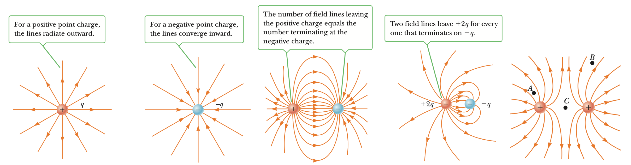
Electric field lines are a common tool that we can use to visualize electric fields.
Conductors vs Insulators
In discussing materials and there response to electric fields, there are often to broad classes of materials. In conductors, electric charges move freely in response to an externally applied electric field. Any material that is not a conductor is referred to as an insulator.
Materials such as glass and rubber are insulators, while materials such as copper and aluminum are good conductors. There are also materials called semiconductors which can act as either conductors or insulators depending on certain stimuli and environmental variables. We will discuss semiconductors in the future.
In the following subsections, we will learn about two different method to electrically charge objects, in addition to some special properties of conductors.
Charging by Conduction
Consider a negatively charged rubber rod brought into contact with an insulated neutral conducting sphere. The excess electrons on the rod repel electrons on the sphere, creating local positive charges on the neutral sphere. On contact, some electrons on the rod are now able to move onto the sphere, thus neutralizing the positive charges. When the rod is removed, the sphere is then left with a net negative charge. This process is referred to as charging by conduction. The object being charged in such a process (in this case, the sphere) is always left with a charge having the same sign as the object doing the charging (in this case, the rubber rod).
Charging by Induction
In contrast to charging by conduction, charging by induction works even when there is no contact between objects. The idea is to create a temporary polarization/dipole (or separation of charges) using a charged objects, and separate the induced dipole such that each half is now is charged. We can illustrate it using the following setup.
Imagine that you have two connected conducting spheres, and a negatively charged object is brought close to the two spheres. Positive charges will accumulate on the left side close to the negatively charged object because opposites attract, while negative charges will accumulate on the right side away from the negatively charged object.
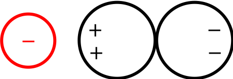
Under the influence of the negatively charged red object, the two spheres become polarized: this means that there is a charge separation with the object itself. When we instantaneously separate the two spheres from one another, the charges will not be able to equilibrate instantaneously, and so the two spheres will therefore become charged, and will remain charged so long as they don’t come into contact with any other conducting objects, even after the red object is removed.
Notice that we were able to charge the spheres even without any physical contact. This is an example of charging by induction.
Electric Fields in Conductors
Consider what happens when we apply an external electric field to a conductor. If there is any field present in the conductor, positive and negative charge densities will separate in response to the field. That separation results in an additional field whose direction is opposite the applied field because of the direction the direction the two polarities of charge move in response to the applied field. This movement occurs until the sum field vanishes, at which point there is no further force on the charges and system becomes static. In other words,
The electric field $\vec{E}=0$ inside any conductor.
Another way to think about it is that if there was any electric field inside the conductor, then the charges on the surface of the conductor would move around because there is an electric force acting on them. Because we are interested in the static equilibrium situation, no charges are moving, and hence no forces are acting on them, meaning there is no internal electric field present.
Another result that can be derived from this conclusion is that
There is no net charge density $\rho$ inside a conductor.
An easy way to prove this is that for a conductor with no net charge, if there was a nonzero $\rho$, then there must be an equal and opposite amount of charge elsewhere in the conductor because the conductor is neutral overall. An electric field would therefore appear between the oppositely signed charge distributions, thereby contradicting the $\vec{E}=0$ condition inside a conductor. This conclusion can be proven more generally for charged conductors, but the argument is easiest to understand and visualize for electrically neutral conductors.
Gauss’s Law
In this section, we will introduce Gauss’s Law, which will turn out to be one of the most useful tools in calculating the electric field due to different charge distributions.
Flux
In order to discuss Gauss’s Law, we first need to understand the mathematical and physical concept of flux. We will take our introduction of flux largely from Purcell and Morin, which is a commonly used introductory electromagnetism textbook for physics majors in college.
Note: In order to understand this material, you must have an understanding of integral calculus in multiple dimensions. If you aren't familiar with multivariable calculus yet, just skip this material.
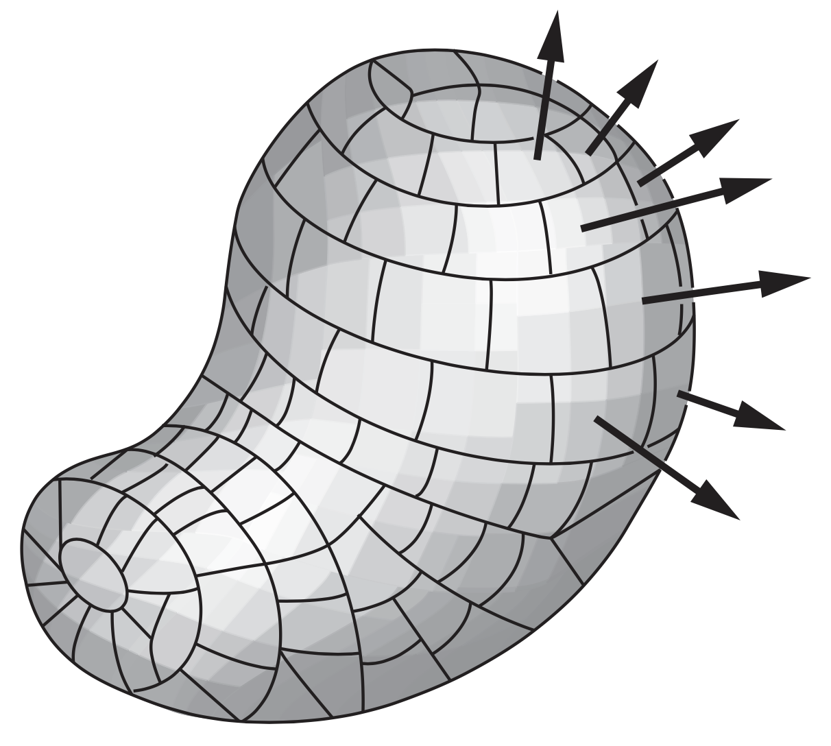
Consider some electric field $\vec{E}$ in space and in this space some arbitrary closed surface, like a balloon of any shape, such as the one shown here.
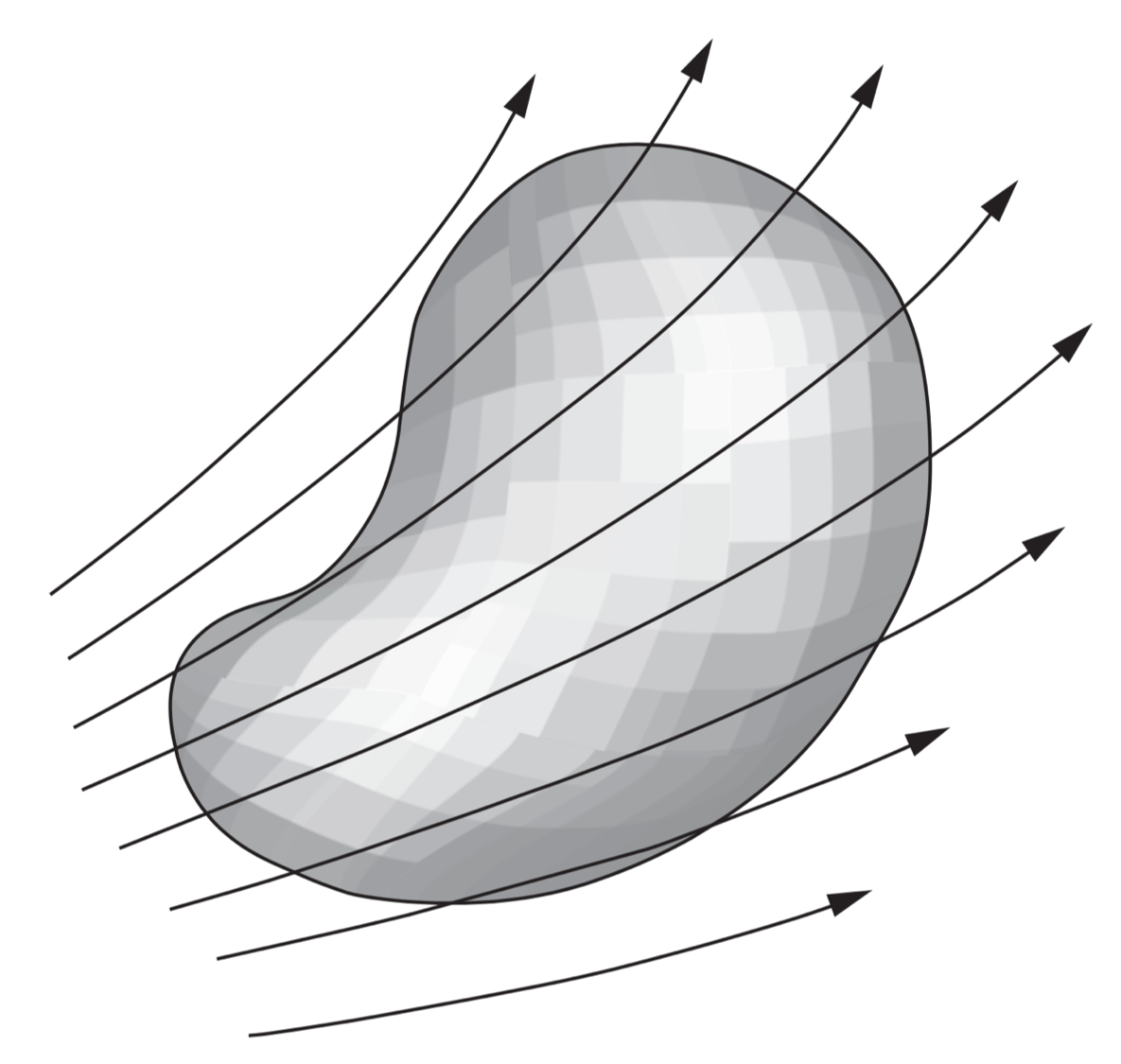
Here, the surface is being exposed to a set of field lines. We can now divide the whole surface into little patches that are so small that over any one path, the surface is practically flat and the vector field does not change appreciably from one part of a patch to another. The area of a patch has a certain magnitude in square meters, and a patch defines a unique direction: the outward-pointing normal vector to its surface. (Since the surface is closed by assumption, you can tell its inside from its outside.) Let this magnitude and direction be represented by a vector $\vec{a}$. Then, for every patch into which the surface has been divided, such as patch number $j$, we have a vector $\vec{a}_j$ giving its area and orientation. The result can be imagined as something like this:
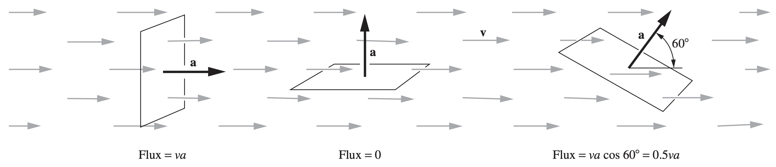
Let $E_j$ be the electric field vector at the location of patch number $j$. The scalar product \(\vec{E}_j \cdot\vec{a}_j\) is a number (review the dot product here). We call this number the flux through that small, infinitesimal bit of surface. We can think of flux as the “rate” of the electric vector field “flowing” into the small area component. The following is a good diagram that illustrate the idea behind flux when calculating the flux of an arbitrary vector field $\vec{v}$ through a surface $\vec{a}$.
In order to calculate the total flux through the entire surface of the balloon due to the electric field, we simply need to add up all of the flux contributions from every single small balloon segment. Let’s denote the total flux as $\Phi$:
\[\Phi=\sum_{\text{all }j}\vec{E}_j\cdot\vec{a}_j\]Of course, in the continuum limit where each of the area segments becomes infinitesimally small, the flux becomes an integral over the entire closed surface:
\[\Phi=\oint_{\mathcal{S}}\vec{E}\cdot d\vec{a}\]The optional material section is now over.
The integral expression above for $\Phi$ is complex. Even if you do have an extensive background in multivariable calculus, no one will ever actually use the integral expression to calculate $\Phi$ from above in real practice. We want an easier method of calculating flux that can be used to calculate flux through common geometrical objects.
Gaussian Surfaces
Imagine that we had a single point charge $q$ at the origin, and some spherical shell surface with some radius $R_0$ that is centered at the origin as well. From our knowledge of the electric field due to a single point charge, we know that the electric field is given by
\[\vec{E}(\vec{r})=\frac{1}{4\pi\varepsilon_0}\frac{q\hat{r}}{r^2}\]Notice that this electric field is always in the radial direction $\hat{r}$, meaning that it is always originating out from the origin, and is therefore always perpendicular to the spherical shell surface. This is nicely illustrated below:
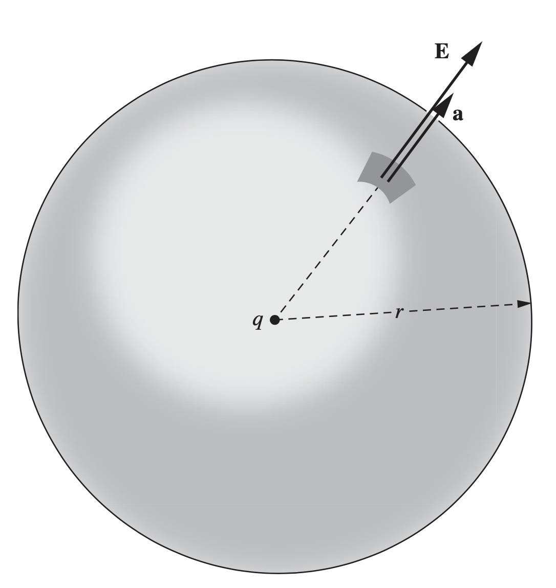
In this case, since $\vec{E}\vert\vert d\vec{a}$ always, the dot product $\vec{E}\cdot d\vec{a}$ is very simply $Eda$. Furthermore, since the radius of the spherical surface is constant and the electric field $\vec{E}$ from above is only dependent on the magnitude of $r^2$, this tells us that the magnitude $E$ is always a constant on the entire surface. In other words, there is no integral for us to actually calculate! The flux “integral” becomes
\[\Phi=\oint_{\mathcal{S}}\vec{E}\cdot d\vec{a}=E\oint_{\mathcal{S}}da=EA\]where $A=4\pi R_0^2$ is simply the total surface area of the spherical shell. Therefore, the flux is simply
\[\Phi=\frac{1}{4\pi\varepsilon_0}\frac{q}{R^2}\cdot 4\pi R^2=\frac{q}{\varepsilon_0}\]Notice that by choosing an appropriate surface – in this case, a spherical shell centered at the point charge – the integral calculation that we had to perform was extremely easy! Such an aptly chosen surface is referred to as a Gaussian surface. Typically we want to chose a surface such that it is always parallel to the direction of the electric field, so that the differential dot product $\vec{E}\cdot d\vec{a}=Eda$ is very easy to calculate. Let’s consider another example with a uniformly applied $\vec{E}$-field $\vec{E}=E_0\hat{z}$ for some constant $E_0$. An easy calculation of flux would be to calculate the flux through, say, a rectangle prism surface with height $h$ and base area $A$.
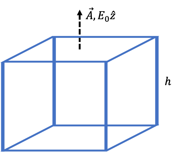
For all of the four sides of the surface that have a side length of $h$, the surfaces are all parallel to the $E_0\hat{z}$ applied field, and so their flux contribution is necessarily zero. However, the top and bottom surfaces, each with area $A$, are perpendicular to the applied electric field, and hence the dot product is once again very easy to calculate. The flux contribution from the top surface is $E_0A$, and the flux contribution from the bottom surface is $-E_0A$. (Note the negative sign! This is because the outwards direction of the area vector $\vec{A}$ is in the $-\hat{z}$ direction instead of the $+\hat{z}$ direction for the bottom surface.) Therefore, the total flux is given by
\[\Phi=E_0A-E_0A+0+0+0+0=0\]Therefore, there is no net flux into or out of this surface!
In general, when trying to compute the flux of the electric field through a closed surface, we often want to pick an appropriate Gaussian surface to make our computation as painless as possible. Although flux is defined by an integral expression, if you find yourself doing anything more complicated than basic multiplication and addition to calculate flux, you’re probably doing something wrong.
The Actual Law
Now that we understand the fundamentals regarding flux and Gaussian surfaces, we can now discuss the actual Gauss’s Law that we were initially interested in. Gauss’s Law often allows us to be able to easily calculate the electric fields of complex charge distributions without just blindly applying Coulomb’s law, and also can be used to calculate a charge distribution given the electric field. Physicists agree that it generally has three primary uses:
- For charge distributions that have some amount of geometrical symmetry, it provides a way to calculate the electric field that is much easier than brute-force integration of Coulomb’s law.
- Gauss’s Law will ultimately prove helpful for us in determining the electric field’s boundary conditions at an interface. We haven’t really discussed what a boundary condition is yet, so don’t worry too much about this point for now.
- If we write Gauss’s Law in differential form (which again, we need to discuss later), we’re able to easily calculate charge densities given that we know what the electric field is.
Gauss’s Law states the following:
Gauss's Law: $\Phi=\oint_{\mathcal{S}}\vec{E}(\vec{r}')\cdot d\vec{a}'=\frac{1}{\varepsilon_0}\int_{\mathcal{V}(\mathcal{S})}d\tau'\rho(\vec{r}')$
Translating this from multivariable calculus to a language that we’re probably more familiar with,
Gauss's Law: $\Phi=EA=\frac{q_{\text{enclosed}}}{\varepsilon_0}$
That is, the flux of the electric field through a Gaussian surface is equal to the total electric charge enclosed in the surface divided by $\varepsilon_0$! We saw an example of the validity of this law above when we calculate the flux $\Phi=q/\varepsilon_0$ through a spherical shell with a point charge source at the center. In the exercises below, we will calculate additional examples to illustrate Gauss’s Law.
A Side Note: Gaussian vs. SI Units
In electromagnetism, unfortunately there are two popular conventions for units and symbolic notations that physicists use: Gaussian-GGS units and SI-MKS units. In introductory physics, SI units are often much more common to come across, so for the purposes of our discussions we will stick to only using SI units unless otherwise stated.
Exercises
Note: None of the exercises below require any use of multivariable calculus (or any calculus, for that matter).
Problem 1
In the early twentieth century, scientist Robert Millikan conducted a well-known set of experiments to try to determine the elementary charge $e$ of the electron. To summarize his experiment, he created a single oil drop of some mass $m$ and carrying a charge of $-q$ ($q<0$), and placed the oil drop between two conducting plates that created a uniform electric field $-E_0\hat{z}$ between the two plates.
- Draw a force diagram that illustrates the forces that are acing on the oil drop.
- Robert Millikan found that for an oil drop that weighed $1$ gram, he needed to apply an electric field of strength $E_0=5.7\times10^{-11}\frac{\text{N}}{\text{C}}$ in order for the oil drop to be suspended and not moving between the two plates. Using an appropriate force balance, calculate the total charge of the oil drop.
- At the time, the mass of the electron was known to be $m_e=9.1\times10^{-31}\text{ kg}$, assuming that the oil drop was entirely composed of electrons, calculate the charge of the electron.
- Compare your result from part 3 to the actual charge of an electron $e$. Are the results similar?
Problem 2
Calculate the electric field at any position $\vec{r}$ due to a hollow conducting spherical shell centered at the origin of radius $R_0$. The shell has a total charge $Q$ that is evenly distributed across its entire two-dimensional surface.
Problem 3
Consider an infinite, non-conducting plane sheet at $z=0$ that has a uniform surface charge density of $\sigma$. Calculate the electric field at any position $\vec{r}$ due to this sheet.
Problem 4
This problem is adapted from Serway Physics 9ed.
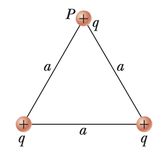
Three equal positive charges are at the corners of an equilateral triangle of side length $a$ as shown above. The three charges $q$ at the corners create an electric field.
- Sketch the electric field lines in the plane of the charges.
- Find the location of one point (other than at infinity) where the electric field is zero.
- What is the electric field at $P$ due to the two charges at the base?