Damped Oscillations
Recall that one of points about the simple harmonic oscillator that we talked about last time that introducing a friction force term that is proportional to the velocity of the mass. We will investigate this situation a bit more closely today.
A quick note: in order to understand all of the (mathematically heavy) derivations, I recommend that you have prior experience with some basic differential equations and have heard of linear independence.
Force Diagram
Our schematic for our mass on a spring setup is exactly the same as it was last time when we introduced the topic of simple harmonic oscillators and Hooke’s Force Law.

Image obtained from Wikimedia Commons.
The setup is the same except that this time, we going to introduce a frictional force term that is equal to $-\gamma\frac{dx}{dt}$. That is, this force is proportional to the velocity of the object, such that $\gamma$ is a constant. The negative sign shows that this force opposes the direction of motion. Physically, these types of force terms don’t really arise from our standard idea of friction between two solid surfaces. A frictional force that is proportional to velocity typically comes from things like air resistance and other types of fluid resistance (for example, if the spring system was emerged in water). Our new force diagram has to account for this:

Here, we have denoted $\vec{F}_f$ as the force of friction. Again, the motion of the mass in the $+\hat{y}$ direction is unremarkable, as we don’t intuitively expect the block to suddenly start jumping around. Applying Newton’s second law in the $+\hat{x}$ direction, we know that
\[ma_x=F_{\text{spring}}+F_f\longrightarrow m\frac{d^2x}{dt^2}=-kx-\gamma\frac{dx}{dt} \longrightarrow \frac{d^2x}{dt^2}+\frac{\gamma}{m}\frac{dx}{dt}+\frac{k}{m}x=0\]This differential equation is called the damped harmonic oscillator equation. We can see that this differential equation boils down to the simple harmonic oscillator equation we discussed last time when $\gamma=0$: that is, when there is no friction force term.
Solving the Damped Harmonic Oscillator Equation
Let’s solve the differential equation we found above for the displacement function $x(t)$, to figure out exactly way the equation describes a damped harmonic oscillator. Taking note that we discussed last week to use an Ansatz involving complex exponentials, we can make a guess that the solution will look something like
\[x(t)=Ae^{i\omega t}+Be^{-i\omega t}\]If we allow for $A$ to be potentially complex, then I assert that we only need to include the first term on the right hand side. You will see why this is below. Therefore, we can have
\[x(t)=Ae^{i\omega t}\]Now, $A$ is potentially complex. Similar to the case with simple harmonic oscillation, we still need to determine what $A$ and $\omega$ are. The first two derivatives of $x(t)$ are
\[\frac{dx}{dt}=Ai\omega e^{i\omega t}, \quad \frac{d^2x}{dt^2}=-A\omega^2 e^{i\omega t}\](Recall that $i^2=-1$.) Plugging these expressions into the differential equation from above gives us
\[-A\omega^2 e^{i\omega t}+A\frac{\gamma i\omega}{m}e^{i\omega t}+A\frac{k}{m}e^{i\omega t}=0\]Let’s factor the left hand side:
\[Ae^{i\omega t}\left(-\omega^2+\frac{\gamma i\omega}{m}+\frac{k}{m}\right)=0\]Because $e^{i\omega t}$ is not always zero for any time point $t$, and we can’t conclude anything about $A$ yet, this tells us that the remaining coefficient must necessarily equal zero:
\[-\omega^2+\frac{\gamma i\omega}{m}+\frac{k}{m}=0\]This is a quadratic equation for $\omega$, so let’s use the quadratic formula to solve this equation:
\[\omega=\frac{\frac{\gamma i}{m}\pm\sqrt{\frac{-\gamma^2}{m^2}+\frac{4k}{m}}}{2}=i\frac{\gamma}{2m}\pm\sqrt{\frac{k}{m}-\left(\frac{\gamma}{2m}\right)^2}\]This is an extremely complicated expression, so let’s break down what’s happening here. $\omega$ is guaranteed to have an imaginary component of $\gamma/2m$. Furthermore, there are actually two allowed solutions: one with the positive sign and one with the negative sign in front of the square root. Both of these are completely valid solutions, and so we should be able to distinguish between the two. Let’s call them $\omega_+$ and $\omega_-$.
\[\omega_+=i\frac{\gamma}{2m}+\sqrt{\frac{k}{m}-\left(\frac{\gamma}{2m}\right)^2}, \quad \omega_-=i\frac{\gamma}{2m}-\sqrt{\frac{k}{m}-\left(\frac{\gamma}{2m}\right)^2}\]The square root contribution is a bit more complicated, as depending on the relative magnitudes of $k, m, \gamma$, we don’t know whether the square root expression is real or imaginary. So, we have to handle each of these cases separately.
Underdamped Solutions
Consider the first case where $\frac{k}{m}-\left(\frac{\gamma}{2m}\right)^2>0$. In our expression for $\omega$ from above, this means that the square root contribution is a real number (since the square root of a positive number is real). Simultaneously, we can relate $\gamma$ and $k$ through this inequality to get $\gamma<\sqrt{4mk}$. In this case, when
\[\gamma<\sqrt{4mk}\]this means that our oscillator is underdamped (we’ll see what this means in a moment). For convenience, we can define $\omega_0=\sqrt{\frac{k}{m}}$ and $\delta \omega=\frac{\gamma}{2m}$. This means that both $\omega_+$ and $\omega_-$ from above can be rewritten as
\[\omega_{\pm}=i\frac{\gamma}{2m}\pm\sqrt{\omega_0^2-(\delta \omega)^2}\]Now that we’ve solved for $\omega$, we need to plug our work back into our complex exponential Ansatz. We determined two possible values of $\omega_+$ and $\omega_-$ that give equally valid solutions, and so we need to factor in both of them. The easiest way to do so is to take a sum of the two solutions. Therefore, the displacement function is given by
\[x(t)=A_+e^{i\omega_+ t}+A_-e^{i\omega_- t}=A_+e^{i^2\gamma t/2m}e^{it\sqrt{\omega_0^2-(\delta\omega)^2}}+A_-e^{i^2t\gamma/2m}e^{-it\sqrt{\omega_0^2-(\delta\omega)^2}}\]Here, $A_+$ and $A_-$ are our arbitrary coefficients that we need to take the take care of later using the initial conditions that we talked about last time. Using the fact that $i^2=-1$, we can further simplify to write
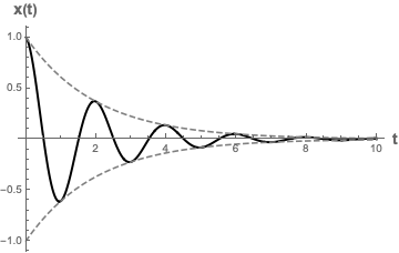
\[x(t)=A_+e^{-\gamma t/2m}e^{it\sqrt{\omega_0^2-(\delta\omega)^2}}+A_-e^{-\gamma t/2m}e^{-it\sqrt{\omega_0^2-(\delta\omega)^2}}\]All of the imaginary components have been explicitly written out in terms of $i$, so we can analyze what’s happening here in more detail. Since $\gamma, m$ are positive and real, the exponential $e^{-\gamma t/2m}$ will result in the exponential decay of the magnitude of the displacement over time. Since the complex exponential terms represent a combination of sine and cosine factors ($e^{iz}=\cos z+i\sin z$), they can be thought of as sinusoidal oscillations with frequency of $\sqrt{\omega_0^2-(\delta\omega)^2}$, similar to the ones that we saw from last time with simple harmonic oscillations. Therefore, together, the solution will appear as an oscillating solution that is damped by an exponential decay factor. To show what this looks like physically, we can set $A_+=2, A_-=2, \gamma=1, m=1, \sqrt{\omega_0^2-(\delta\omega)^2}=\pi$ and plot the resulting graph of $x(t)$ as a function of $t$.
Overdamped Solutions
Now, lets consider another case where $\frac{k}{m}-\left(\frac{\gamma}{2m}\right)^2<0$. This means that
\[\gamma>\sqrt{4mk}\]We refer to this as an overdamped oscillator. Again, we’ll use the same notations conversions as above: $\omega_0=\sqrt{\frac{k}{m}}$ and $\delta\omega=\frac{\gamma}{2m}$. Because of the assumed relation between $\gamma, m, k$, this means that
\[\omega_{\pm}=i\frac{\gamma}{2m}\pm i\sqrt{(\delta \omega)^2-\omega_0^2}\]Plugging this again into our complex exponential Ansatz, and again summing both the $\omega_+$ and $\omega_-$ solution, we find (after simplification) that
\[x(t)=A_+\exp\left[-t\left(\delta \omega+\sqrt{(\delta \omega)^2-\omega_0^2}\right)\right]+A_-\exp\left[-t\left(\delta \omega-\sqrt{(\delta \omega)^2-\omega_0^2}\right)\right]\]Again, this isn’t a math class. We are interested in what this solution means physically. In this case, the solution looks almost exactly like the solution in the underdamped case, but without the sinusoidal, complex exponential term. We only have the exponential decay factor in this case. To find out what this looks like physically, let’s try setting $A_+=1, A_-=0, \delta\omega=5, \omega_0=4$ using some arbitrary set of units and plot what the resulting function looks like:
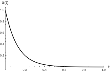
In this overdamped case, there’s no oscillations: the displacement from the equilibrium length of the spring just decays to zero rapidly.
Critically Damped
In this final case study, let’s examine the final possible case where $\frac{k}{m}-\left(\frac{\gamma}{2m}\right)^2=0$. In other words, we have
\[\gamma=\sqrt{4mk}\]In this case, the square root term doesn’t contribute to the expression for $\omega_{\pm}$, and so we have
\[\omega_+=\omega_-=\frac{\gamma}{2m}\]Therefore, we can conclude that
\[x(t)=Ae^{-\gamma t/2m}\]Well, technically this isn’t quite true. In the very special case that $\gamma=\sqrt{4mk}$, there is actually another possible solution to the damped harmonic oscillator equation: $x(t)=Bte^{-\gamma t/2m}$. To prove this is also a solution, I recommend you plug this Ansatz into the damped harmonic oscillator equation and confirm it for yourself. Or, you can just take my word for it ![]() . Therefore, in order to describe the full solution, we need to actually take the sum of both of these possible solutions. The correct general solution in this case is therefore
. Therefore, in order to describe the full solution, we need to actually take the sum of both of these possible solutions. The correct general solution in this case is therefore
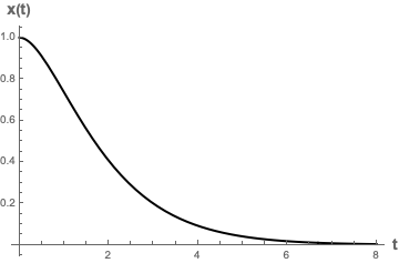
Again, to gain some sort of physical intuition of what this graph looks like, we can set $A=B=1, \gamma=2, m=1$ to see what the resulting solution functionally looks like:
Getting a Feel for the Solutions
Let’s recap what we’ve learned from above by examining each of the three cases once more:
- Underdamped Oscillation: $\gamma<\sqrt{4mk}$. In this case, the frictional force is weak enough (compared to the restorative spring force) such that the mass can oscillate a few times, but due to the friction, energy is being sapped away from the system and the mass will eventually stop oscillating. The general solution (in complex exponential form) is \(x(t)=A_+e^{-\gamma t/2m}e^{it\sqrt{\omega_0^2-(\delta\omega)^2}}+A_-e^{-\gamma t/2m}e^{-it\sqrt{\omega_0^2-(\delta\omega)^2}}\), where $A_+$ and $A_-$ are fixed by the initial conditions of the system.
- Critically Damped Oscillation: $\gamma=\sqrt{4mk}$. In this case, the frictional force is just enough when compared to the spring force such that the mass doesn’t oscillate, but rather just decays back to its original rest equilibrium position. Moreover, the frictional force isn’t so overwhelming that its stoping the restorative spring force from returning to its equilibrium position. The friction and spring forces are “in balance” so that the mass comes right back to its original equilibrium position and then stops moving.
- Overdamped Oscillation: $\gamma>\sqrt{4mk}$. In this case, the frictional force is so strong (compared to the restorative spring force) such that the mass can’t even return to the equilibrium position quickly because the strong friction force is overpowering the restorative spring force. The mass will eventually return to its equilibrium position, just much more slowly.
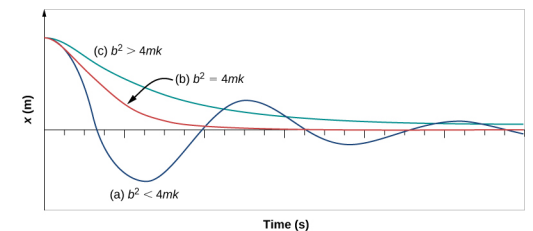
You might have guessed already, but given the same initial conditions, mass, and spring but just varying the friction parameter $\gamma$, the critically damped mass will return to its equilibrium position, and stay there, the fastest. The underdamped mass will oscillate many times before returning to equilibrium, and the overdamped mass will slowly return before returning to equilibrium. Here’s an excellent comparative diagram from Physics Libretexts:
While understanding the different forms of the solutions and how we derive them mathematically is important, having a feel of the intuition behind each of the three different systems is even more important. This link provides an excellent simulation on the different forms of solutions. I strongly encourage you to check it out.
What’s the Real Solution?
Mathematically, we’ve determined what the solution to the damped harmonic oscillator equation is in different cases of relating $\gamma, k, m$. However, remember that we’re dealing with physical quantities here: things like displacement and time are real. Therefore, our final answer shouldn’t involve any imaginary terms, because it doesn’t make sense that displacement should have an imaginary component.
One way of overcoming this is by simply taking the real part of the solution at the end of the problem before boxing the final solution. Take the real part after plugging in the initial conditions and everything. This will give the valid solution.
Another option is to not use complex exponential form. In this case, although it is a little bit more difficult to derive, another valid Ansatz to make is of the form
\[x(t)=Ae^{-\gamma t/2m}\cos(\omega t+\delta)\]Here, we still have to determine what $\omega$, $A$, and $\delta$ are based on the premises of the problem. We’ve seen what $\omega$ and $A$ are. $\delta$ is called the phase factor and refers to some constant. In an exercise below, you will prove that this real Ansatz and taking the real part of the complex exponential form Ansatz from above yield exactly the same result.
Appendix: Using Only One Basis Function
Recall that from above, we asserted that our complex exponential solution had the general form of $x(t)=Ae^{i\omega t}+Be^{-i\omega t}$. When then stated that we could neglect the $Be^{-i\omega t}$ part of the solution. To prove this consider the case where $x(t)=Be^{-i\omega t}$. Plugging this into the damped harmonic oscillator equation gives us
\[-B\omega^2e^{-i\omega t}-B\frac{\gamma i\omega}{m}e^{-i\omega t}+B\frac{k}{m}e^{-i\omega t}=0\]Factoring the left hand side gives
\[Be^{-i\omega t}\left(-\omega^2-\frac{\gamma i\omega}{m}+\frac{k}{m}\right)=0 \longrightarrow -\omega^2-\frac{\gamma i\omega}{m}+\frac{k}{m}=0\]We can use the quadratic formula to solve this equation for $\omega$. After simplifying the algebra, we have
\[\omega=-i\frac{\gamma}{2m} \pm \sqrt{\frac{k}{m}-\left(\frac{\gamma}{2m}\right)^2}\]The important part of the solution that we are concerned about is the $-i\frac{\gamma}{2m}$ component. If we plug this part of $\omega$ back into the general form solution, we have
\[x(t)=Be^{-i^2t\gamma/2m}=Be^{t\gamma/2m}\]Compare this with our work for above involving the $e^{i\omega t}$ case. Here, we have an exponential term $e^{t\gamma/2m}$ that is modifying the amplitude of the potential oscillation of the mass of the block by essentially saying that the block’s oscillation exponentially increases with increasing time, resulting in an infinite amount of energy and work. When modeling a system with friction, this clearly makes no sense. Therefore, although the $Be^{-i\omega t}$ part of the solution is mathematically correct, we must discard it because it makes no physical sense.
Exercises
Problem 1
In our work from above, we asserted that another valid Ansatz to make is of the form
\[x(t)=Ae^{-\gamma t/2m}\cos(\omega t+\delta)\]Answer the following questions.
- By plugging this Ansatz into the damped harmonic oscillator equation, show that this is indeed the correct form for a general solution to the general damped harmonic oscillator setup. What is $\omega$?
- Suppose that a mass starts at the initial position $x_0=1$ at time $t=0$, with initial velocity $v_0=0$ in some arbitrary units. Solve for the parameters $A, \delta$ using the form of the solution above given these initial conditions. Take $\gamma=2, k=2, m=1$ for some arbitrary units.
- Using the same initial conditions from part (2) of this problem, solve for the parameters $A$ in the complex exponential form of the solution. Remember that here, $A$ can be complex. Once again, take $\gamma=2, k=2, m=1$ for some arbitrary units.
- Are your solutions from parts (2) and (3) the same?
Problem 2
Consider a mass on an inclined plane attached to a spring.
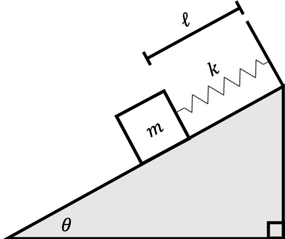
The spring has an equilibrium length $\ell$.
- Draw a free body diagram for the mass $m$ in this system.
- Assume that there is no friction between the mass and the inclined plane. Solve for the motion of the block.
- Assume that the block is not yet moving and the maximum force of static friction is defined to be $-\mu_s N$, where $N$ is the normal force and $\mu_s$ is the coefficient of static friction. What is the maximum distance from the top of the inclined plane that the block can be before it begins to move?
- Assume that the force of friction is instead defined to be $-\gamma \frac{dx}{dt}$, and there is no $-\mu_s N$ type friction present. Solve for the motion of the block given that the mass starts at its equilibrium length with velocity $v_0$ at time $t=0$. Assume that $\gamma=2, k=1, m=1$ for some set or arbitrary units.
Problem 3
This problem is adapted from Serway Physics, Ninth Edition.
A 3.00-kg object is fastened to a light spring, with the intervening cord passing over a pulley.
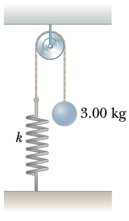
The pulley is frictionless, and its inertia may be neglected. The object is released from rest when the spring is unstretched. If the object drops 10.0 cm before stopping, find
- the spring constant of the spring.
- the speed of the object when it is 5.00 cm below its starting point.
Problem 4
This problem is adapted from Caltech’s Physics 1a Course.
A large block of mass $m_1$ executes horizontal simple harmonic motion as it slides across a frictionless surface under the action of a spring constant $k$. A block of mass $m_2$ rests upon $m_1$. The coefficient of friction between the two blocks is $\mu$. Assume that $m_2$ does not slip relative to $m_1$.
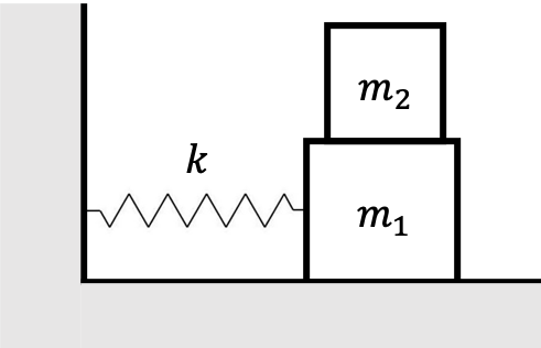
Answer the following questions about this setup.
- Draw the free body diagrams for $m_1$ and $m_2$ at a time when the spring is stretched a distance $x$ beyond equilibrium to the right.
- Write down the horizontal and vertical equations of motion for blocks $m_1$ and $m_2$.
- What is the angular frequncy of oscillation, $\omega$, of the system?
- What is the maximum amplitude of oscillation, $A$, that the system can have if $m_2$ is not to slip relative to $m_1$? (Write your answer in terms of $\omega$.)